Chapter 11 | Stage 3: Map generation
Once the model is run through the three proposed phases, we have all the information required for generating the maps. We need to transform the output vector to raster layers. We will obtain the SOC stocks after 20 years of SSM practices for the three scenarios (low, medium and high carbon inputs increments), and SOC stocks under the business as usual scenario (no carbon input increment). We will estimate four absolute carbon sequestration rates (considering the 2018 or 2020 SOC as a baseline), and three relative carbon sequestration rates (considering the SOC stocks under the business as usual as the baseline).
11.1 Script Number 16: “Points_to_Raster.R”
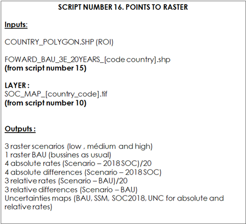
We will use script number 16 to transform the output vector from script number 15 to raster layers. The inputs for this script are the output vector from script 15, the FAO SOC layer and the country boundary polygon. The outputs of the script number 16 are the SOC stocks for the future scenarios (20 years): BAU, low, medium and high carbon inputs, three relative sequestration rates (SOC stock SSM scenario - BAU scenario)/20 , and four absolute sequestration rates: (SOC stock SSM or BAU scenario - SOC stocks 2018/20)/20.
Table 11.1 Script Number 16. Target Points to Rasters Products. Inputs and Outputs
We will open the script “Points_to_Raster.R” and load the required packages; then set the directories of the required files: Forward outputs, SOC, AOI, and the outputs maps folder.
rm(list=ls())
library(raster)
library(rgdal)
WD_F<-("C:/TRAINING_MATERIALS_GSOCseq_MAPS_28-09-2020/OUTPUTS/3_FOWARD")
WD_SOC<-("C:/TRAINING_MATERIALS_GSOCseq_MAPS_28-09-2020/INPUTS/SOC_MAP")
WD_AOI<-("C:/TRAINING_MATERIALS_GSOCseq_MAPS_28-09-2020/INPUTS/AOI_POLYGON")
WD_MAPS<-("C:/TRAINING_MATERIALS_GSOCseq_MAPS_28-09-2020/OUTPUTS/4_MAPS")
Now we will define the name of the output area of interest / country or region. In this example, “Pergamino”.
#Define the name of the Country ("ISO3CountryCode")
name<-"Pergamino"
Then open the layers:
#Open FORWARD vector
setwd(WD_F)
FOWARD<-readOGR("FOWARD_County_AOI.shp")
#Open SOC MAP (master layer)
setwd(WD_SOC)
SOC_MAP<-raster("SOC_MAP_AOI.tif")
#Creates emtpy raster
empty_raster<-SOC_MAP*0
# Open the country vector boundaries
setwd(WD_AOI)
Country<-readOGR("Departamento_Pergamino.shp")
# Cut the raster with the country vector
Country_raster<-crop(empty_raster,Country)
# Replace Na values for zero values
FOWARD@data[is.na(FOWARD@data)] <- 0
Next, we will transform the vector points from the FORWARD phase of the model to raster files using the “rasterize” function.
# Points to Raster BAU
setwd(WD_MAPS)
Country_BAU_2040_Map<-rasterize(FOWARD, Country_raster ,FOWARD$SOC_BAU_20, updateValue='all')
writeRaster(Country_BAU_2040_Map,filename=paste0(name,"_GSOCseq_finalSOC_BAU_Map030"),format="GTiff")
# Points to Raster Low Scenario
Country_Lwr_2040_Map<-rasterize(FOWARD, Country_raster ,FOWARD$Lw_Sc, updateValue='all')
writeRaster(Country_Lwr_2040_Map,filename=paste0(name,"_GSOCseq_finalSOC_SSM1_Map030"),format="GTiff")
# Points to Raster Med Scenario
Country_Med_2040_Map<-rasterize(FOWARD, Country_raster ,FOWARD$Md_Sc, updateValue='all')
writeRaster(Country_Med_2040_Map,filename=paste0(name,"_GSOCseq_finalSOC_SSM2_Map030"),format="GTiff")
# Points to Raster High Scenario
Country_Hgh_2040_Map<-rasterize(FOWARD, Country_raster ,FOWARD$Hgh_S, updateValue='all')
writeRaster(Country_Hgh_2040_Map,filename=paste0(name,"_GSOCseq_finalSOC_SSM3_Map030"),format="GTiff")

# Points to Raster initial SOC (t0) 2018/2020
Country_SOC_2018_Map<-rasterize(FOWARD, Country_raster ,FOWARD$SOC__, updateValue='all')
writeRaster(Country_SOC_2018_Map,filename=paste0(name,"_GSOCseq_T0_Map030"),format="GTiff")
Now, we will calculate the absolute differences and the absolute rates (SSM - SOC 2018).
# Difference BAU 2040 - SOC 2018
Diff_BAU_SOC_2018<-Country_BAU_2040_Map-Country_SOC_2018_Map
writeRaster(Diff_BAU_SOC_2018,filename=paste0(name,"_GSOCseq_AbsDiff_BAU_Map030"),format="GTiff")
writeRaster(Diff_BAU_SOC_2018/20,filename=paste0(name,"_GSOCseq_ASR_BAU_Map030"),format="GTiff")
# Difference Low Scenario - SOC 2018
Diff_Lw_SOC_2018<-Country_Lwr_2040_Map-Country_SOC_2018_Map
writeRaster(Diff_Lw_SOC_2018,filename=paste0(name,"_GSOCseq_AbsDiff_SSM1_Map030"),format="GTiff")
writeRaster(Diff_Lw_SOC_2018/20,filename=paste0(name,"_GSOCseq_ASR_SSM1_Map030"),format="GTiff")
# Difference Med Scenario - SOC 2018
Diff_Md_SOC_2018<-Country_Med_2040_Map-Country_SOC_2018_Map
writeRaster(Diff_Md_SOC_2018,filename=paste0(name,"_GSOCseq_AbsDiff_SSM2_Map030"),format="GTiff")
writeRaster(Diff_Md_SOC_2018/20,filename=paste0(name,"_GSOCseq_ASR_SSM2_Map030"),format="GTiff")
# Difference High Scenario - SOC 2018
Diff_Hg_SOC_2018<-Country_Hgh_2040_Map-Country_SOC_2018_Map
writeRaster(Diff_Hg_SOC_2018,filename=paste0(name,"_GSOCseq_AbsDiff_SSM3_Map030"),format="GTiff")
writeRaster(Diff_Hg_SOC_2018/20,filename=paste0(name,"_GSOCseq_ASR_SSM3_Map030"),format="GTiff")
Next, we will calculate the relative differences and rates (SSM - SOC BAU).
# Difference Low Scenario - BAU 2040
Diff_Lw_BAU_2040<-Country_Lwr_2040_Map-Country_BAU_2040_Map
writeRaster(Diff_Lw_BAU_2040,filename=paste0(name,"_GSOCseq_RelDiff_SSM1_Map030"),format="GTiff")
writeRaster(Diff_Lw_BAU_2040/20,filename=paste0(name,"_GSOCseq_RSR_SSM1_Map030"),format="GTiff")
# Difference Med Scenario - BAU 2040
Diff_Md_BAU_2040<-Country_Med_2040_Map-Country_BAU_2040_Map
writeRaster(Diff_Md_BAU_2040,filename=paste0(name,"_GSOCseq_RelDiff_SSM2_Map030"),format="GTiff")
writeRaster(Diff_Md_BAU_2040/20,filename=paste0(name,"_GSOCseq_RSR_SSM2_Map030"),format="GTiff")
# Difference High Scenario - BAU 2040
Diff_Hg_BAU_2040<-Country_Hgh_2040_Map-Country_BAU_2040_Map
writeRaster(Diff_Hg_BAU_2040,filename=paste0(name,"_GSOCseq_RelDiff_SSM3_Map030"),format="GTiff")
writeRaster(Diff_Hg_BAU_2040/20,filename=paste0(name,"_GSOCseq_RSR_SSM3_Map030"),format="GTiff")
Now, we will rasterize the values of the uncertainties of SOC BAU, SOC 2018 and one SSM (one for the three scenarios).
# Uncertainties SOC 2018
UNC_2018<-rasterize(FOWARD, Country_raster ,FOWARD$UNC_2, updateValue='all')
writeRaster(UNC_2018,filename=paste0(name,"_GSOCseq_T0_UncertaintyMap030"),format="GTiff")
# Uncertainties SOC BAU 2038
UNC_BAU<-rasterize(FOWARD, Country_raster ,FOWARD$UNC_B, updateValue='all')
writeRaster(UNC_BAU,filename=paste0(name,"_GSOCseq_BAU_UncertaintyMap030"),format="GTiff")
# Uncertainties SOC SSM
UNC_SSM<-rasterize(FOWARD, Country_raster ,FOWARD$UNC_S, updateValue='all')
writeRaster(UNC_SSM,filename=paste0(name,"_GSOCseq_SSM_UncertaintyMap030"),format="GTiff")
Now we will calculate the uncertainties for the absolute rates.
# Uncertainties for the Absolute difference SSM_ - SOC2018
UNC_abs_rate_BAU<-sqrt((FOWARD$UNC_B*FOWARD$SOC_BAU_20)^2+ (FOWARD$UNC_2*FOWARD$SOC__)^2)/abs(FOWARD$SOC__+FOWARD$SOC_BAU_20)
UNC_abs_rate_BAU_Map<-rasterize(FOWARD,Country_raster,UNC_abs_rate_BAU, updateValue='all')
writeRaster(UNC_abs_rate_BAU_Map,filename=paste0(name,"_GSOCseq_ASR_BAU_UncertaintyMap030"),format="GTiff")
UNC_abs_rate_Lw<-sqrt((FOWARD$UNC_S*FOWARD$Lw_Sc)^2 + (FOWARD$UNC_2*FOWARD$SOC__)^2)/abs(FOWARD$SOC__+FOWARD$Lw_Sc)
UNC_abs_rate_Lw_Map<-rasterize(FOWARD,Country_raster,UNC_abs_rate_Lw, updateValue='all')
writeRaster(UNC_abs_rate_Lw_Map,filename=paste0(name,"_GSOCseq_ASR_SSM1_UncertaintyMap030"),format="GTiff")

UNC_abs_rate_Md<-sqrt((FOWARD$UNC_S*FOWARD$Md_Sc)^2+ (FOWARD$UNC_2*FOWARD$SOC__)^2)/abs(FOWARD$SOC__+FOWARD$Md_Sc)
UNC_abs_rate_Md_Map<-rasterize(FOWARD,Country_raster,UNC_abs_rate_Md, updateValue='all')
writeRaster(UNC_abs_rate_Md_Map,filename=paste0(name,"_GSOCseq_ASR_SSM2_UncertaintyMap030"),format="GTiff")
UNC_abs_rate_Hg<-sqrt((FOWARD$UNC_S*FOWARD$Hgh_S)^2 + (FOWARD$UNC_2*FOWARD$SOC__)^2)/abs(FOWARD$SOC__+FOWARD$Hgh_S)
UNC_abs_rate_Hg_Map<-rasterize(FOWARD,Country_raster,UNC_abs_rate_Hg, updateValue='all')
writeRaster(UNC_abs_rate_Hg_Map,filename=paste0(name,"_GSOCseq_ASR_SSM3_UncertaintyMap030"),format="GTiff")
Now we will calculate the uncertainties for the relative rates.
# Uncertainties for the Relative difference  SSM_ - SOCBAU
UNC_Rel_rate_Lw<-sqrt((FOWARD$UNC_S*FOWARD$Lw_Sc)^2+ (FOWARD$UNC_B*FOWARD$SOC_BAU_20)^2)/abs(FOWARD$SOC_BAU_20+FOWARD$Lw_Sc)
UNC_Rel_rate_Lw_Map<-rasterize(FOWARD,Country_raster,UNC_Rel_rate_Lw, updateValue='all')
writeRaster(UNC_Rel_rate_Lw_Map,filename=paste0(name,"_GSOCseq_RSR_SSM1_UncertaintyMap030"),format="GTiff")
UNC_Rel_rate_Md<-sqrt((FOWARD$UNC_S*FOWARD$Md_Sc)^2+ (FOWARD$UNC_B*FOWARD$SOC_BAU_20)^2)/abs(FOWARD$SOC_BAU_20+FOWARD$Md_Sc)
UNC_Rel_rate_Md_Map<-rasterize(FOWARD,Country_raster,UNC_Rel_rate_Md, updateValue='all')
writeRaster(UNC_Rel_rate_Md_Map,filename=paste0(name,"_GSOCseq_RSR_SSM2_UncertaintyMap030"),format="GTiff")

UNC_Rel_rate_Hg<-sqrt((FOWARD$UNC_S*FOWARD$Hgh_S)^2+ (FOWARD$UNC_B*FOWARD$SOC_BAU_20)^2)/abs(FOWARD$SOC_BAU_20+FOWARD$Hgh_S)
UNC_Rel_rate_Hg_Map<-rasterize(FOWARD,Country_raster,UNC_Rel_rate_Hg, updateValue='all')
writeRaster(UNC_Rel_rate_Hg_Map,filename=paste0(name,"_GSOCseq_RSR_SSM3_UncertaintyMap030"),format="GTiff")