Annex I Troubleshooting
Coastal and small countries not fully covered by the CRU layers
Due to the coarse resolution of the CRU layers a lot of points close to the country boarders can be lost (Figure 15.1).
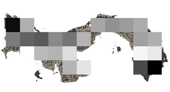
Figure 15.1 Points outside of a given CRU layer for Panama.
To overcome this, we provided two options:
- Perform the whole procedure with higher resolution climate layers again for every point. We have provided scripts to download and prepare TerraClimate climatic layers.
- Prepare the CRU layers with the newly provided scripts that include a line of code that fills NA values with the average of the three nearest pixel values. If you have already completed all steps, you can repeat the procedure solely for points that fall outside the CRU layer.
In the following a small guide for option 2 on how to select and run the model for points that fall outside the CRU layers is provided:
Step 1 Create a single CRU layer cropped and masked to the extent of your AOI using the following R script
#+++++++++++++++++++++++++++++++++++++++++
#  DATE:  02/03/2021                     #
#                                        #
#  Isabel Luotto                         #
#                                        #
# This script can be used to clip        #
# one of the CRU layers                  #
# to the shape of the AOI                #
#                                        #
#+++++++++++++++++++++++++++++++++++++++++

#Empty environment
rm(list = ls())

#Load libraries
library(raster)
library(rgdal)

#Define paths to the single folder locations
WD_AOI<-("C:/TRAINING_MATERIALS_GSOCseq_MAPS_12-11-2020/INPUTS/AOI_POLYGON")
WD_CRU<-("C:/TRAINING_MATERIALS_GSOCseq_MAPS_12-11-2020/INPUTS/CRU_LAYERS")

#Load any of the CRU tif layers created with script N. 1
setwd(WD_CRU)
CRU <- raster("PET_Stack_01-18_CRU.tif")

#Load your AOI shapefile
setwd(WD_AOI)
AOI <- readOGR("PAN_adm0.shp")

#Crop and mask CRU layer
CRU<-crop(CRU,AOI)
CRU<-mask(CRU,AOI)

#Save cropped masked raster layer
setwd(WD_CRU)
writeRaster(CRU, "CRU_AOI_QGIS.tif" )
Step 2 Open QGIS and generate the empty points
- Repeat section 9.5.1 QGIS Procedure number 1 (model) in the technical manual to generate the empty points
- Load the cropped CRU layer created previously
Step 3 Polygonize the raster
- Go to.. Raster/Conversion/Polygonize (Raster to Vector)
- Select CRU layer as input and click on Run (Figure 15.2)
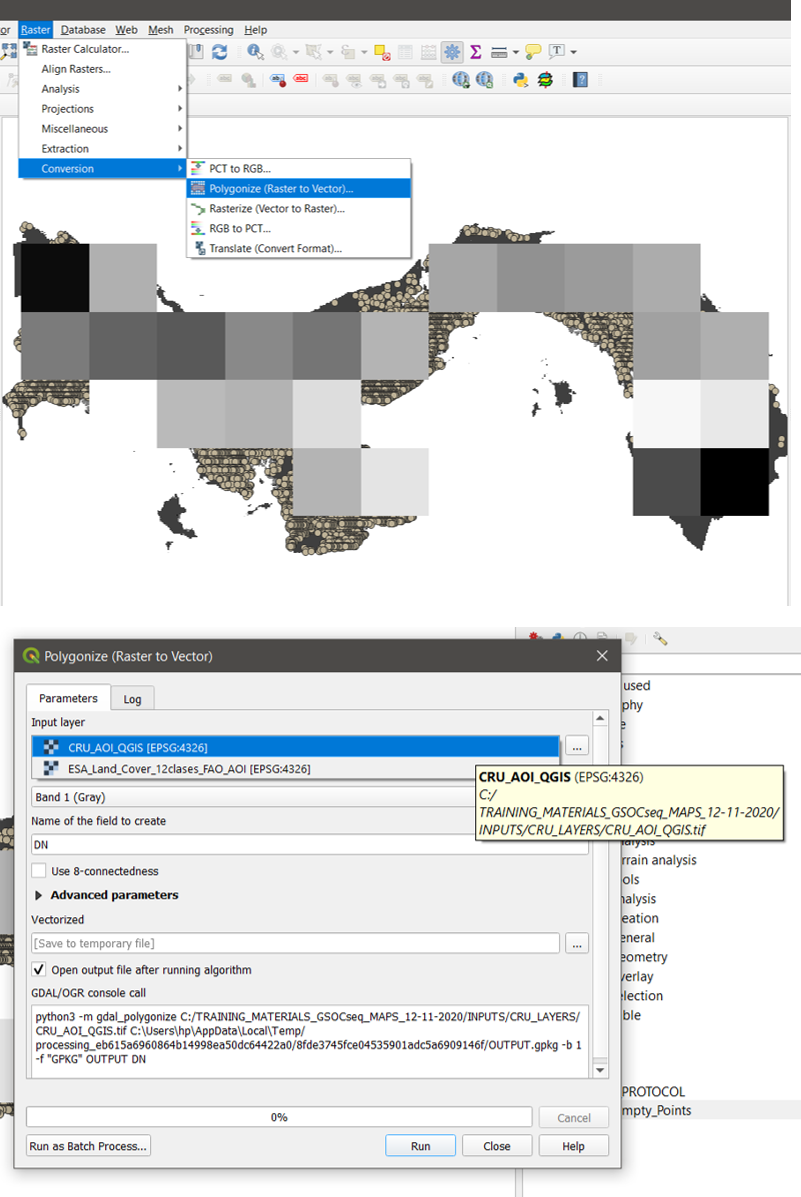
Figure 15.2 Raster to Vector
Step 4 Select points outside of the polygon
- Type: “select by location” in the processing toolbox search bar and open the Select by Location tool
- Select the Points as input and click on the disjoint check box and click on Run (Figure 15.3)
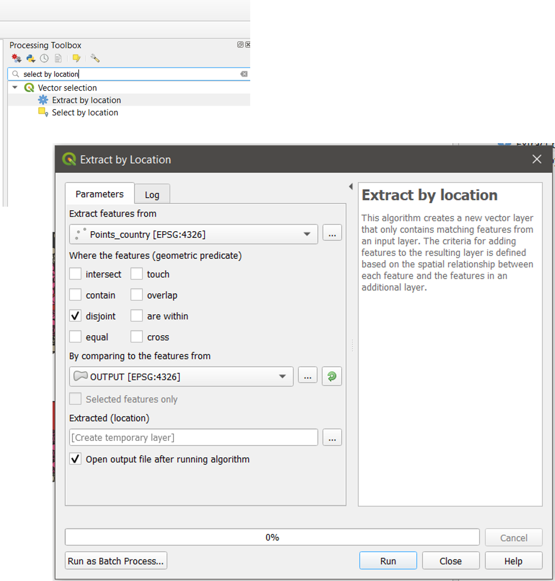
Figure 15.3 Select points outside a polygon
Step 5 Export the extracted points
- Right click on the newly created layer. Got to Export/Save Features As “AOI_Empty_points_borders” (Figure 15.3)

Figure 15.3 Export the extracted points
Step 6 Run the Spin up phase for points outside the CRU layer (Script 13B)
Scripts 13B, 14B and 15B are modified versions of script 13 (Spin up phase), 14 (Warm up phase) and 15 (Forward phase) which include lines of code that fill NA pixel values from the CRU layers with the average of all surrounding pixel values. The same raster stacks created for the original map can be used as input to run the model over the points that fall outside the CRU layers.
#12/11/2020

# SPATIAL SOIL R  for VECTORS

###### SPIN UP ################

# MSc Ing Agr Luciano E Di Paolo
# Dr Ing Agr Guillermo E Peralta
###################################
# SOilR from Sierra, C.A., M. Mueller, S.E. Trumbore (2012).
#Models of soil organic matter decomposition: the SoilR package, version 1.0 Geoscientific Model Development, 5(4),
#1045--1060. URL http://www.geosci-model-dev.net/5/1045/2012/gmd-5-1045-2012.html.
#####################################

rm(list=ls())

library(SoilR)
library(raster)
library(rgdal)
library(soilassessment)


# Set working directory

WD_FOLDER<-("D:/TRAINING_MATERIALS_GSOCseq_MAPS_12-11-2020")

# Vector must be an empty points vector.

setwd(WD_FOLDER)
Vector<-readOGR("INPUTS/TARGET_POINTS/AOI_Empty_points_borders.shp")

# Stack_Set_1 is a stack that contains the spatial variables

Stack_Set_1<- stack("INPUTS/STACK/Stack_Set_SPIN_UP_AOI.tif")

# Add pixels to the borders to avoid removing coastal areas

for (i in 1:nlayers(Stack_Set_1)){
  Stack_Set_1[[i]]<-focal(Stack_Set_1[[i]], w = matrix(1,25,25), fun= mean,  na.rm = TRUE, NAonly=TRUE , pad=TRUE)
}

# Create A vector to save the results

C_INPUT_EQ<-Vector

# use this only for backup

# C_INPUT_EQ<-readOGR("OUTPUTS/1_SPIN_UP/SPIN_UP_BSAS_27-03-2020_332376.shp")

# extract variables to points

Vector_variables<-extract(Stack_Set_1,Vector,df=TRUE)

# Extract the layers from the Vector

SOC_im<-Vector_variables[[2]] # primera banda del stack

clay_im<-Vector_variables[[3]] # segunda banda del stack

DR_im<-Vector_variables[[40]]

LU_im<-Vector_variables[[41]]

# Define Years for Cinputs calculations

years=seq(1/12,500,by=1/12)

# ROTH C MODEL FUNCTION .

########## function set up starts###############
Roth_C<-function(Cinputs,years,DPMptf, RPMptf, BIOptf, HUMptf, FallIOM,Temp,Precip,Evp,Cov,Cov1,Cov2,soil.thick,SOC,clay,DR,bare1,LU)

{

# Paddy fields coefficent fPR = 0.4 if the target point is class = 13 , else fPR=1
# From Shirato and Yukozawa 2004

fPR=(LU == 13)*0.4 + (LU!=13)*1

#Temperature effects per month
fT=fT.RothC(Temp[,2])

#Moisture effects per month .

fw1func<-function(P, E, S.Thick = 30, pClay = 32.0213, pE = 1, bare)
{

    M = P - E * pE
    Acc.TSMD = NULL
    for (i in 2:length(M)) {
    B = ifelse(bare[i] == FALSE, 1, 1.8)
     Max.TSMD = -(20 + 1.3 * pClay - 0.01 * (pClay^2)) * (S.Thick/23) * (1/B)
        Acc.TSMD[1] = ifelse(M[1] > 0, 0, M[1])
        if (Acc.TSMD[i - 1] + M[i] < 0) {
            Acc.TSMD[i] = Acc.TSMD[i - 1] + M[i]
        }
        else (Acc.TSMD[i] = 0)
        if (Acc.TSMD[i] <= Max.TSMD) {
            Acc.TSMD[i] = Max.TSMD
        }
    }
    b = ifelse(Acc.TSMD > 0.444 * Max.TSMD, 1, (0.2 + 0.8 * ((Max.TSMD -
        Acc.TSMD)/(Max.TSMD - 0.444 * Max.TSMD))))
    b<-clamp(b,lower=0.2)
    return(data.frame(b))
}

fW_2<- fw1func(P=(Precip[,2]), E=(Evp[,2]), S.Thick = soil.thick, pClay = clay, pE = 1, bare=bare1)$b

#Vegetation Cover effects

fC<-Cov2[,2]

# Set the factors frame for Model calculations

xi.frame=data.frame(years,rep(fT*fW_2*fC*fPR,length.out=length(years)))

# RUN THE MODEL from soilassessment
#Roth C soilassesment
Model3_spin=carbonTurnover(tt=years,C0=c(DPMptf, RPMptf, BIOptf, HUMptf, FallIOM),In=Cinputs,Dr=DR,clay=clay,effcts=xi.frame, "euler")
Ct3_spin=Model3_spin[,2:6]

# RUN THE MODEL FROM SOILR
#Model3_spin=RothCModel(t=years,C0=c(DPMptf, RPMptf, BIOptf, HUMptf, FallIOM),In=Cinputs,DR=DR,clay=clay,xi=xi.frame, pass=TRUE)
#Ct3_spin=getC(Model3_spin)

# Get the final pools of the time series
poolSize3_spin=as.numeric(tail(Ct3_spin,1))

return(poolSize3_spin)
}
########## function set up ends###############

# Iterates over the area of interest

########for loop starts###############3
for (i in 1:dim(Vector_variables)[1]) {

# Extract the variables

Vect<-as.data.frame(Vector_variables[i,])

Temp<-as.data.frame(t(Vect[4:15]))
Temp<-data.frame(Month=1:12, Temp=Temp[,1])

Precip<-as.data.frame(t(Vect[16:27]))
Precip<-data.frame(Month=1:12, Precip=Precip[,1])

Evp<-as.data.frame(t(Vect[28:39]))
Evp<-data.frame(Month=1:12, Evp=Evp[,1])

Cov<-as.data.frame(t(Vect[42:53]))
Cov1<-data.frame(Cov=Cov[,1])
Cov2<-data.frame(Month=1:12, Cov=Cov[,1])

#Avoid calculus over Na values

if (any(is.na(Evp[,2])) | any(is.na(Temp[,2])) | any(is.na(SOC_im[i])) | any(is.na(clay_im[i])) | any(is.na(Precip[,2]))  |  any(is.na(Cov2[,2]))  |  any(is.na(Cov1[,1]))  | any(is.na(DR_im[i])) |  (SOC_im[i]<0) | (clay_im[i]<0) ) {C_INPUT_EQ[i,2]<-0}else{

# Set the variables from the images

soil.thick=30  #Soil thickness (organic layer topsoil), in cm
SOC<-SOC_im[i]      #Soil organic carbon in Mg/ha
clay<-clay_im[i]        #Percent clay %

DR<-DR_im[i]              # DPM/RPM (decomplosable vs resistant plant material.)
bare1<-(Cov1>0.8)           # If the surface is bare or vegetated
LU<-LU_im[i]

#IOM using Falloon method
FallIOM=0.049*SOC^(1.139)

# If you use a SOC uncertainty layer turn on this. First open the layer SOC_UNC
#(it must have the same extent and resolution of the SOC layer)

#SOC_min<-(1-(SOC_UNC/100))*SOC
#SOC_max<-(1+(SOC_UNC/100))*SOC

# Define SOC min, max Clay min and max.
SOC_min<-SOC*0.8
SOC_max<-SOC*1.2
clay_min<-clay*0.9
clay_max<-clay*1.1

b<-1

# C input equilibrium. (Ceq)

fb<-Roth_C(Cinputs=b,years=years,DPMptf=0, RPMptf=0, BIOptf=0, HUMptf=0, FallIOM=FallIOM,Temp=Temp,Precip=Precip,Evp=Evp,Cov=Cov,Cov1=Cov1,Cov2=Cov2,soil.thick=soil.thick,SOC=SOC,clay=clay,DR=DR,bare1=bare1,LU=LU)
fb_t<-fb[1]+fb[2]+fb[3]+fb[4]+fb[5]

m<-(fb_t-FallIOM)/(b)

Ceq<-(SOC-FallIOM)/m

# UNCERTAINTIES C input equilibrium (MINIMUM)
FallIOM_min=0.049*SOC_min^(1.139)

fb_min<-Roth_C(Cinputs=b,years=years,DPMptf=0, RPMptf=0, BIOptf=0, HUMptf=0, FallIOM=FallIOM,Temp=Temp*1.02,Precip=Precip*0.95,Evp=Evp,Cov=Cov,Cov1=Cov1,Cov2=Cov2,soil.thick=soil.thick,SOC=SOC_min,clay=clay_min,DR=DR,bare1=bare1,LU=LU)
fb_t_MIN<-fb_min[1]+fb_min[2]+fb_min[3]+fb_min[4]+fb_min[5]

m<-(fb_t_MIN-FallIOM_min)/(b)

Ceq_MIN<-(SOC_min-FallIOM_min)/m

# UNCERTAINTIES C input equilibrium (MAXIMUM)
FallIOM_max=0.049*SOC_max^(1.139)

fb_max<-Roth_C(Cinputs=b,years=years,DPMptf=0, RPMptf=0, BIOptf=0, HUMptf=0, FallIOM=FallIOM,Temp=Temp*0.98,Precip=Precip*1.05,Evp=Evp,Cov=Cov,Cov1=Cov1,Cov2=Cov2,soil.thick=soil.thick,SOC=SOC_max,clay=clay_max,DR=DR,bare1=bare1,LU=LU)
fb_t_MAX<-fb_max[1]+fb_max[2]+fb_max[3]+fb_max[4]+fb_max[5]

m<-(fb_t_MAX-FallIOM_max)/(b)

Ceq_MAX<-(SOC_max-FallIOM_max)/m

# SOC POOLS AFTER 500 YEARS RUN WITH C INPUT EQUILIBRIUM

if (LU==2 | LU==12 | LU==13){
RPM_p_2<-((0.184*SOC + 0.1555)*(clay + 1.275)^(-0.1158))*0.9902+0.4788
BIO_p_2<-((0.014*SOC + 0.0075)*(clay + 8.8473)^(0.0567))*1.09038+0.04055
HUM_p_2<-((0.7148*SOC + 0.5069)*(clay + 0.3421)^(0.0184))*0.9878-0.3818
DPM_p_2<-SOC-FallIOM-RPM_p_2-HUM_p_2-BIO_p_2

feq_t<-RPM_p_2+BIO_p_2+HUM_p_2+DPM_p_2+FallIOM

#uncertainties  MIN

RPM_p_2_min<-((0.184*SOC_min + 0.1555)*(clay_min + 1.275)^(-0.1158))*0.9902+0.4788
BIO_p_2_min<-((0.014*SOC_min + 0.0075)*(clay_min + 8.8473)^(0.0567))*1.09038+0.04055
HUM_p_2_min<-((0.7148*SOC_min + 0.5069)*(clay_min + 0.3421)^(0.0184))*0.9878-0.3818
DPM_p_2_min<-SOC_min-FallIOM_min-RPM_p_2_min-HUM_p_2_min-BIO_p_2_min

feq_t_min<-RPM_p_2_min+BIO_p_2_min+HUM_p_2_min+DPM_p_2_min+FallIOM_min

#uncertainties  MAX

RPM_p_2_max<-((0.184*SOC_max + 0.1555)*(clay_max + 1.275)^(-0.1158))*0.9902+0.4788
BIO_p_2_max<-((0.014*SOC_max + 0.0075)*(clay_max + 8.8473)^(0.0567))*1.09038+0.04055
HUM_p_2_max<-((0.7148*SOC_max + 0.5069)*(clay_max + 0.3421)^(0.0184))*0.9878-0.3818
DPM_p_2_max<-SOC_max-FallIOM_max-RPM_p_2_max-HUM_p_2_max-BIO_p_2_max

feq_t_max<-RPM_p_2_max+BIO_p_2_max+HUM_p_2_max+DPM_p_2_max+FallIOM_max

C_INPUT_EQ[i,2]<-SOC
C_INPUT_EQ[i,3]<-Ceq
C_INPUT_EQ[i,4]<-feq_t
C_INPUT_EQ[i,5]<-DPM_p_2
C_INPUT_EQ[i,6]<-RPM_p_2
C_INPUT_EQ[i,7]<-BIO_p_2
C_INPUT_EQ[i,8]<-HUM_p_2
C_INPUT_EQ[i,9]<-FallIOM
C_INPUT_EQ[i,10]<-Ceq_MIN
C_INPUT_EQ[i,11]<-Ceq_MAX
C_INPUT_EQ[i,12]<-feq_t_min
C_INPUT_EQ[i,13]<-DPM_p_2_min
C_INPUT_EQ[i,14]<-RPM_p_2_min
C_INPUT_EQ[i,15]<-BIO_p_2_min
C_INPUT_EQ[i,16]<-HUM_p_2_min
C_INPUT_EQ[i,17]<-FallIOM_min
C_INPUT_EQ[i,18]<-feq_t_max
C_INPUT_EQ[i,19]<-DPM_p_2_max
C_INPUT_EQ[i,20]<-RPM_p_2_max
C_INPUT_EQ[i,21]<-BIO_p_2_max
C_INPUT_EQ[i,22]<-HUM_p_2_max
C_INPUT_EQ[i,23]<-FallIOM_max

}else if(LU==4){

RPM_p_4<-((0.184*SOC + 0.1555)*(clay + 1.275)^(-0.1158))*1.7631+0.4043
BIO_p_4<-((0.014*SOC + 0.0075)*(clay + 8.8473)^(0.0567))*0.9757+0.0209
HUM_p_4<-((0.7148*SOC + 0.5069)*(clay + 0.3421)^(0.0184))*0.8712-0.2904
DPM_p_4<-SOC-FallIOM-RPM_p_4-HUM_p_4-BIO_p_4

feq_t<-RPM_p_4+BIO_p_4+HUM_p_4+DPM_p_4+FallIOM

#uncertainties min

RPM_p_4_min<-((0.184*SOC_min + 0.1555)*(clay_min + 1.275)^(-0.1158))*1.7631+0.4043
BIO_p_4_min<-((0.014*SOC_min + 0.0075)*(clay_min + 8.8473)^(0.0567))*0.9757+0.0209
HUM_p_4_min<-((0.7148*SOC_min + 0.5069)*(clay_min + 0.3421)^(0.0184))*0.8712-0.2904
DPM_p_4_min<-SOC_min-FallIOM_min-RPM_p_4_min-HUM_p_4_min-BIO_p_4_min

feq_t_min<-RPM_p_4_min+BIO_p_4_min+HUM_p_4_min+DPM_p_4_min+FallIOM_min

#uncertainties max

RPM_p_4_max<-((0.184*SOC_max + 0.1555)*(clay_max + 1.275)^(-0.1158))*1.7631+0.4043
BIO_p_4_max<-((0.014*SOC_max + 0.0075)*(clay_max + 8.8473)^(0.0567))*0.9757+0.0209
HUM_p_4_max<-((0.7148*SOC_max + 0.5069)*(clay_max + 0.3421)^(0.0184))*0.8712-0.2904
DPM_p_4_max<-SOC_max-FallIOM_max-RPM_p_4_max-HUM_p_4_max-BIO_p_4_max

feq_t_max<-RPM_p_4_max+BIO_p_4_max+HUM_p_4_max+DPM_p_4_max+FallIOM_max

C_INPUT_EQ[i,2]<-SOC
C_INPUT_EQ[i,3]<-Ceq
C_INPUT_EQ[i,4]<-feq_t
C_INPUT_EQ[i,5]<-DPM_p_4
C_INPUT_EQ[i,6]<-RPM_p_4
C_INPUT_EQ[i,7]<-BIO_p_4
C_INPUT_EQ[i,8]<-HUM_p_4
C_INPUT_EQ[i,9]<-FallIOM
C_INPUT_EQ[i,10]<-Ceq_MIN
C_INPUT_EQ[i,11]<-Ceq_MAX
C_INPUT_EQ[i,12]<-feq_t_min
C_INPUT_EQ[i,13]<-DPM_p_4_min
C_INPUT_EQ[i,14]<-RPM_p_4_min
C_INPUT_EQ[i,15]<-BIO_p_4_min
C_INPUT_EQ[i,16]<-HUM_p_4_min
C_INPUT_EQ[i,17]<-FallIOM_min
C_INPUT_EQ[i,18]<-feq_t_max
C_INPUT_EQ[i,19]<-DPM_p_4_max
C_INPUT_EQ[i,20]<-RPM_p_4_max
C_INPUT_EQ[i,21]<-BIO_p_4_max
C_INPUT_EQ[i,22]<-HUM_p_4_max
C_INPUT_EQ[i,23]<-FallIOM_max

} else if (LU==3 | LU==5 | LU==6 | LU==8){

RPM_p_3<-((0.184*SOC + 0.1555)*(clay + 1.275)^(-0.1158))*1.3837+0.4692
BIO_p_3<-((0.014*SOC + 0.0075)*(clay + 8.8473)^(0.0567))*1.03401+0.02531
HUM_p_3<-((0.7148*SOC + 0.5069)*(clay + 0.3421)^(0.0184))*0.9316-0.5243
DPM_p_3<-SOC-FallIOM-RPM_p_3-HUM_p_3-BIO_p_3

feq_t<-RPM_p_3+BIO_p_3+HUM_p_3+DPM_p_3+FallIOM

#uncertainties min

RPM_p_3_min<-((0.184*SOC_min + 0.1555)*(clay_min + 1.275)^(-0.1158))*1.3837+0.4692
BIO_p_3_min<-((0.014*SOC_min + 0.0075)*(clay_min + 8.8473)^(0.0567))*1.03401+0.02531
HUM_p_3_min<-((0.7148*SOC_min + 0.5069)*(clay_min + 0.3421)^(0.0184))*0.9316-0.5243
DPM_p_3_min<-SOC_min-FallIOM_min-RPM_p_3_min-HUM_p_3_min-BIO_p_3_min

feq_t_min<-RPM_p_3_min+BIO_p_3_min+HUM_p_3_min+DPM_p_3_min+FallIOM_min

#uncertainties max

RPM_p_3_max<-((0.184*SOC_max + 0.1555)*(clay_max + 1.275)^(-0.1158))*1.3837+0.4692
BIO_p_3_max<-((0.014*SOC_max + 0.0075)*(clay_max + 8.8473)^(0.0567))*1.03401+0.02531
HUM_p_3_max<-((0.7148*SOC_max + 0.5069)*(clay_max + 0.3421)^(0.0184))*0.9316-0.5243
DPM_p_3_max<-SOC_max-FallIOM_max-RPM_p_3_max-HUM_p_3_max-BIO_p_3_max

feq_t_max<-RPM_p_3_max+BIO_p_3_max+HUM_p_3_max+DPM_p_3_max+FallIOM_max


C_INPUT_EQ[i,2]<-SOC
C_INPUT_EQ[i,3]<-Ceq
C_INPUT_EQ[i,4]<-feq_t
C_INPUT_EQ[i,5]<-DPM_p_3
C_INPUT_EQ[i,6]<-RPM_p_3
C_INPUT_EQ[i,7]<-BIO_p_3
C_INPUT_EQ[i,8]<-HUM_p_3
C_INPUT_EQ[i,9]<-FallIOM
C_INPUT_EQ[i,10]<-Ceq_MIN
C_INPUT_EQ[i,11]<-Ceq_MAX
C_INPUT_EQ[i,12]<-feq_t_min
C_INPUT_EQ[i,13]<-DPM_p_3_min
C_INPUT_EQ[i,14]<-RPM_p_3_min
C_INPUT_EQ[i,15]<-BIO_p_3_min
C_INPUT_EQ[i,16]<-HUM_p_3_min
C_INPUT_EQ[i,17]<-FallIOM_min
C_INPUT_EQ[i,18]<-feq_t_max
C_INPUT_EQ[i,19]<-DPM_p_3_max
C_INPUT_EQ[i,20]<-RPM_p_3_max
C_INPUT_EQ[i,21]<-BIO_p_3_max
C_INPUT_EQ[i,22]<-HUM_p_3_max
C_INPUT_EQ[i,23]<-FallIOM_max

}else {
C_INPUT_EQ[i,2]<-SOC
C_INPUT_EQ[i,3]<-Ceq
C_INPUT_EQ[i,4]<-0
C_INPUT_EQ[i,5]<-0
C_INPUT_EQ[i,6]<-0
C_INPUT_EQ[i,7]<-0
C_INPUT_EQ[i,8]<-0
C_INPUT_EQ[i,9]<-0
C_INPUT_EQ[i,10]<-0
C_INPUT_EQ[i,11]<-0
C_INPUT_EQ[i,12]<-0
C_INPUT_EQ[i,13]<-0
C_INPUT_EQ[i,14]<-0
C_INPUT_EQ[i,15]<-0
C_INPUT_EQ[i,16]<-0
C_INPUT_EQ[i,17]<-0
C_INPUT_EQ[i,18]<-0
C_INPUT_EQ[i,19]<-0
C_INPUT_EQ[i,20]<-0
C_INPUT_EQ[i,21]<-0
C_INPUT_EQ[i,22]<-0
C_INPUT_EQ[i,23]<-0

}

print(c(i,SOC,Ceq))

}
}
###############for loop ends##############


#rename de columns

colnames(C_INPUT_EQ@data)[2]="SOC_FAO"
colnames(C_INPUT_EQ@data)[3]="Cinput_EQ"
colnames(C_INPUT_EQ@data)[4]="SOC_pedotransfer"
colnames(C_INPUT_EQ@data)[5]="DPM_pedotransfer"
colnames(C_INPUT_EQ@data)[6]="RPM_pedotransfer"
colnames(C_INPUT_EQ@data)[7]="BIO_pedotransfer"
colnames(C_INPUT_EQ@data)[8]="HUM_pedotransfer"
colnames(C_INPUT_EQ@data)[9]="IOM_pedotransfer"
colnames(C_INPUT_EQ@data)[10]="CIneq_min"
colnames(C_INPUT_EQ@data)[11]="CIneq_max"
colnames(C_INPUT_EQ@data)[12]="SOC_min"
colnames(C_INPUT_EQ@data)[13]="DPM_min"
colnames(C_INPUT_EQ@data)[14]="RPM_min"
colnames(C_INPUT_EQ@data)[15]="BIO_min"
colnames(C_INPUT_EQ@data)[16]="HUM_min"
colnames(C_INPUT_EQ@data)[17]="IOM_min"
colnames(C_INPUT_EQ@data)[18]="SOC_max"
colnames(C_INPUT_EQ@data)[19]="DPM_max"
colnames(C_INPUT_EQ@data)[20]="RPM_max"
colnames(C_INPUT_EQ@data)[21]="BIO_max"
colnames(C_INPUT_EQ@data)[22]="HUM_max"
colnames(C_INPUT_EQ@data)[23]="IOM_max"

# SAVE the Points (shapefile)

setwd("D:/TRAINING_MATERIALS_GSOCseq_MAPS_12-11-2020/OUTPUTS/1_SPIN_UP")
writeOGR(C_INPUT_EQ, ".", "SPIN_UP_County_AOI", driver="ESRI Shapefile",overwrite=TRUE)
Step 7 Run the Warm up phase for points outside the CRU layer (Script 14B)
#12/11/2020

# SPATIAL SOIL R  for VECTORS

#   ROTH C phase 3: WARM UP

# MSc Ing Agr Luciano E Di Paolo
# Dr Ing Agr Guillermo E Peralta
###################################
# SOilR from Sierra, C.A., M. Mueller, S.E. Trumbore (2012).
#Models of soil organic matter decomposition: the SoilR package, version 1.0 Geoscientific Model Development, 5(4),
#1045--1060. URL http://www.geosci-model-dev.net/5/1045/2012/gmd-5-1045-2012.html.
#####################################

rm(list=ls())

library(SoilR)
library(raster)
library(rgdal)
library(soilassessment)

working_dir<-setwd("D:/TRAINING_MATERIALS_GSOCseq_MAPS_12-11-2020")

#Open empty vector

Vector<-readOGR("INPUTS/TARGET_POINTS/AOI_Empty_points_borders.shp")

#Open Warm Up Stack

Stack_Set_warmup<- stack("INPUTS/STACK/Stack_Set_WARM_UP_AOI.tif")

# Add pixels to the borders to avoid removing costal areas

for (i in 1:nlayers(Stack_Set_warmup)){
  Stack_Set_warmup[[i]]<-focal(Stack_Set_warmup[[i]], w = matrix(1,25,25), fun= mean,  na.rm = TRUE, NAonly=TRUE , pad=TRUE)
}

# Open Result from SPIN UP PROCESS. A vector with 5 columns , one for each pool

Spin_up<-readOGR("D:/TRAINING_MATERIALS_GSOCseq_MAPS_12-11-2020/OUTPUTS/1_SPIN_UP/SPIN_UP_County_AOI.shp")
Spin_up<-as.data.frame(Spin_up)

# Open Precipitation , temperature, and EVapotranspiration file 20 anios x 12 = 240 layers x 3

# CRU LAYERS
PREC<-stack("INPUTS/CRU_LAYERS/Prec_Stack_216_01-18_CRU.tif")
TEMP<-stack("INPUTS/CRU_LAYERS/Temp_Stack_216_01-18_CRU.tif")
PET<-stack("INPUTS/CRU_LAYERS/PET_Stack_216_01-18_CRU.tif")

for (i in 1:nlayers(PREC)){
  PREC[[i]]<-focal(PREC[[i]], w = matrix(1,3,3), fun= mean,  na.rm = TRUE, NAonly=TRUE , pad=TRUE)
}
for (i in 1:nlayers(TEMP)){
  TEMP[[i]]<-focal(TEMP[[i]], w = matrix(1,3,3), fun= mean,  na.rm = TRUE, NAonly=TRUE , pad=TRUE)
}

for (i in 1:nlayers(PET)){
  PET[[i]]<-focal(PET[[i]], w = matrix(1,3,3), fun= mean,  na.rm = TRUE, NAonly=TRUE , pad=TRUE)
}


# TERRA CLIMATE LAYERS
#PREC<-stack("INPUTS/TERRA_CLIME/Precipitation_2001-2021_Pergamino.tif")
#TEMP<-stack("INPUTS/TERRA_CLIME/AverageTemperature_2001-2021_Pergamino.tif")*0.1
#PET<-stack("INPUTS/TERRA_CLIME/PET_2001-2021_Pergamino.tif")*0.1

#Open Mean NPP MIAMI 1981 - 2000

NPP<-raster("INPUTS/NPP/NPP_MIAMI_MEAN_81-00_AOI.tif")
NPP<-focal(NPP, w = matrix(1,3,3), fun= mean,  na.rm = TRUE, NAonly=TRUE , pad=TRUE)

NPP_MEAN_MIN<-raster("INPUTS/NPP/NPP_MIAMI_MEAN_81-00_AOI_MIN.tif")
NPP_MEAN_MIN<-focal(NPP_MEAN_MIN, w = matrix(1,3,3), fun= mean,  na.rm = TRUE, NAonly=TRUE , pad=TRUE)

NPP_MEAN_MAX<-raster("INPUTS/NPP/NPP_MIAMI_MEAN_81-00_AOI_MAX.tif")
NPP_MEAN_MAX<-focal(NPP_MEAN_MAX, w = matrix(1,3,3), fun= mean,  na.rm = TRUE, NAonly=TRUE , pad=TRUE)

#Open LU layer (year 2000).

LU_AOI<-raster("INPUTS/LAND_USE/ESA_Land_Cover_12clases_FAO_AOI.tif")

#Apply NPP coeficientes
NPP<-(LU_AOI==2 | LU_AOI==12 | LU_AOI==13)*NPP*0.53+ (LU_AOI==4)*NPP*0.88 + (LU_AOI==3 | LU_AOI==5 | LU_AOI==6 | LU_AOI==8)*NPP*0.72
NPP_MEAN_MIN<-(LU_AOI==2 | LU_AOI==12 | LU_AOI==13)*NPP_MEAN_MIN*0.53+ (LU_AOI==4)*NPP_MEAN_MIN*0.88 + (LU_AOI==3 | LU_AOI==5 | LU_AOI==6 | LU_AOI==8)*NPP_MEAN_MIN*0.72
NPP_MEAN_MAX<-(LU_AOI==2 | LU_AOI==12 | LU_AOI==13)*NPP_MEAN_MAX*0.53+ (LU_AOI==4)*NPP_MEAN_MAX*0.88 + (LU_AOI==3 | LU_AOI==5 | LU_AOI==6 | LU_AOI==8)*NPP_MEAN_MAX*0.72


# Extract variables to points

Vector_points<-extract(Stack_Set_warmup,Vector,sp=TRUE)
Vector_points<-extract(TEMP,Vector_points,sp=TRUE)
Vector_points<-extract(PREC,Vector_points,sp=TRUE)
Vector_points<-extract(PET,Vector_points,sp=TRUE)
Vector_points<-extract(NPP,Vector_points,sp=TRUE)
Vector_points<-extract(NPP_MEAN_MIN,Vector_points,sp=TRUE)
Vector_points<-extract(NPP_MEAN_MAX,Vector_points,sp=TRUE)

WARM_UP<-Vector

#use only for backup

#WARM_UP<-readOGR("WARM_UP_County_AOI3_97.shp")

# Warm Up number of years simulation

yearsSimulation<-dim(TEMP)[3]/12

clim_layers<-yearsSimulation*12

nppBand<-nlayers(Stack_Set_warmup)+clim_layers*3+2

firstClimLayer<-nlayers(Stack_Set_warmup)+2

nppBand_min<-nppBand+1

nppBand_max<-nppBand+2

nDR_beg<-(16+yearsSimulation)
nDR_end<-nDR_beg+(yearsSimulation-1)

# Extract the layers from the Vector

SOC_im<-Vector_points[[2]]

clay_im<-Vector_points[[3]]

LU_im<-Vector_points[[16]]

NPP_im<-Vector_points[[nppBand]]

NPP_im_MIN<-Vector_points[[nppBand_min]]

NPP_im_MAX<-Vector_points[[nppBand_max]]

# Define Years

years=seq(1/12,1,by=1/12)


# ROTH C MODEL FUNCTION .

###########function set up starts################
Roth_C<-function(Cinputs,years,DPMptf, RPMptf, BIOptf, HUMptf, FallIOM,Temp,Precip,Evp,Cov,Cov1,Cov2,soil.thick,SOC,clay,DR,bare1,LU)

{

# Paddy fields coefficent fPR = 0.4 if the target point is class = 13 , else fPR=1
# From Shirato and Yukozawa 2004

fPR=(LU == 13)*0.4 + (LU!=13)*1

#Temperature effects per month
fT=fT.RothC(Temp[,2])

#Moisture effects per month . Si se usa evapotranspiracion pE=1

fw1func<-function(P, E, S.Thick = 30, pClay = 32.0213, pE = 1, bare)
{

    M = P - E * pE
    Acc.TSMD = NULL
    for (i in 2:length(M)) {
    B = ifelse(bare[i] == FALSE, 1, 1.8)
     Max.TSMD = -(20 + 1.3 * pClay - 0.01 * (pClay^2)) * (S.Thick/23) * (1/B)
        Acc.TSMD[1] = ifelse(M[1] > 0, 0, M[1])
        if (Acc.TSMD[i - 1] + M[i] < 0) {
            Acc.TSMD[i] = Acc.TSMD[i - 1] + M[i]
        }
        else (Acc.TSMD[i] = 0)
        if (Acc.TSMD[i] <= Max.TSMD) {
            Acc.TSMD[i] = Max.TSMD
        }
    }
    b = ifelse(Acc.TSMD > 0.444 * Max.TSMD, 1, (0.2 + 0.8 * ((Max.TSMD -
        Acc.TSMD)/(Max.TSMD - 0.444 * Max.TSMD))))
    b<-clamp(b,lower=0.2)
    return(data.frame(b))
}


fW_2<- fw1func(P=(Precip[,2]), E=(Evp[,2]), S.Thick = soil.thick, pClay = clay, pE = 1, bare=bare1)$b

#Vegetation Cover effects  C1: No till Agriculture, C2: Conventional Agriculture, C3: Grasslands and Forests, C4 bareland and Urban

fC<-Cov2[,2]

# Set the factors frame for Model calculations

xi.frame=data.frame(years,rep(fT*fW_2*fC*fPR,length.out=length(years)))

# RUN THE MODEL from SoilR
#Loads the model Si pass=TRUE genera calcula el modelo aunque sea invalido.
#Model3_spin=RothCModel(t=years,C0=c(DPMptf, RPMptf, BIOptf, HUMptf, FallIOM),In=Cinputs,DR=DR,clay=clay,xi=xi.frame, pass=TRUE)
#Calculates stocks for each pool per month
#Ct3_spin=getC(Model3_spin)

# RUN THE MODEL from soilassesment

Model3_spin=carbonTurnover(tt=years,C0=c(DPMptf, RPMptf, BIOptf, HUMptf, FallIOM),In=Cinputs,Dr=DR,clay=clay,effcts=xi.frame, "euler")

Ct3_spin=Model3_spin[,2:6]

# Get the final pools of the time series

poolSize3_spin=as.numeric(tail(Ct3_spin,1))

return(poolSize3_spin)

}
##############funtion set up ends##########

# Iterates over the area of interest and over 18 years

Cinputs<-c()
Cinputs_min<-c()
Cinputs_max<-c()
NPP_M_MIN<-c()
NPP_M_MAX<-c()
NPP_M<-c()

############for loop starts################
for (i in 1:(length(Vector_points))) {

gt<-firstClimLayer
gp<-gt+clim_layers
gevp<-gp+clim_layers

for (w in 1:(dim(TEMP)[3]/12)) {

print(c("year:",w))
# Extract the variables

Vect<-as.data.frame(Vector_points[i,])

Temp<-as.data.frame(t(Vect[gt:(gt+11)]))
Temp<-data.frame(Month=1:12, Temp=Temp[,1])

Precip<-as.data.frame(t(Vect[gp:(gp+11)]))
Precip<-data.frame(Month=1:12, Precip=Precip[,1])

Evp<-as.data.frame(t(Vect[gevp:(gevp+11)]))
Evp<-data.frame(Month=1:12, Evp=Evp[,1])

Cov<-as.data.frame(t(Vect[4:15]))
Cov1<-data.frame(Cov=Cov[,1])
Cov2<-data.frame(Month=1:12, Cov=Cov[,1])

DR_im<-as.data.frame(t(Vect[nDR_beg:nDR_end])) # DR one per year according to LU
DR_im<-data.frame(DR_im=DR_im[,1])

gt<-gt+12
gp<-gp+12
gevp<-gevp+12

#Avoid calculus over Na values

if (any(is.na(Evp[,2])) | any(is.na(Temp[,2])) | any(is.na(SOC_im[i])) | any(is.na(clay_im[i])) | any(is.na(Spin_up[i,3]))  | any(is.na(NPP_im[i])) | any(is.na(Precip[,2]))  |  any(is.na(Cov2[,2]))  |  any(is.na(Cov1[,1]))  | any(is.na(DR_im[,1]))    |  (SOC_im[i]<0) | (clay_im[i]<0) | (Spin_up[i,3]<=0) ) {WARM_UP[i,2]<-0}else{

# Get the variables from the vector

soil.thick=30  #Soil thickness (organic layer topsoil), in cm
SOC<-SOC_im[i]      #Soil organic carbon in Mg/ha
clay<-clay_im[i]        #Percent clay %

DR<-DR_im[w,1]              # DPM/RPM (decomplosable vs resistant plant material.)
bare1<-(Cov1>0.8)           # If the surface is bare or vegetated
NPP_81_00<-NPP_im[i]
NPP_81_00_MIN<-NPP_im_MIN[i]
NPP_81_00_MAX<-NPP_im_MAX[i]

# PHASE 2  : WARM UP .  years (w)

# Cinputs
T<-mean(Temp[,2])
P<-sum(Precip[,2])
NPP_M[w]<-NPPmodel(P,T,"miami")*(1/100)*0.5
NPP_M[w]<-(LU_im[i]==2 | LU_im[i]==12 | LU_im[i]==13)*NPP_M[w]*0.53+ (LU_im[i]==4)*NPP_M[w]*0.88 + (LU_im[i]==3 | LU_im[i]==5 | LU_im[i]==6 | LU_im[i]==8)*NPP_M[w]*0.72

if (w==1) {Cinputs[w]<-(Spin_up[i,3]/NPP_81_00)*NPP_M[w]} else {Cinputs[w]<-(Cinputs[[w-1]]/ NPP_M[w-1]) * NPP_M[w]}

# Cinputs MIN

Tmin<-mean(Temp[,2]*1.02)
Pmin<-sum(Precip[,2]*0.95)
NPP_M_MIN[w]<-NPPmodel(Pmin,Tmin,"miami")*(1/100)*0.5
NPP_M_MIN[w]<-(LU_im[i]==2 | LU_im[i]==12 | LU_im[i]==13)*NPP_M_MIN[w]*0.53+ (LU_im[i]==4)*NPP_M_MIN[w]*0.88 + (LU_im[i]==3 | LU_im[i]==5 | LU_im[i]==6 | LU_im[i]==8)*NPP_M_MIN[w]*0.72

if (w==1) {Cinputs_min[w]<-(Spin_up[i,10]/NPP_81_00)*NPP_M_MIN[w]} else {Cinputs_min[w]<-(Cinputs_min[[w-1]]/ NPP_M_MIN[w-1]) * NPP_M_MIN[w]}

# Cinputs MAX

Tmax<-mean(Temp[,2]*0.98)
Pmax<-sum(Precip[,2]*1.05)
NPP_M_MAX[w]<-NPPmodel(Pmax,Tmax,"miami")*(1/100)*0.5
NPP_M_MAX[w]<-(LU_im[i]==2 | LU_im[i]==12 | LU_im[i]==13)*NPP_M_MAX[w]*0.53+ (LU_im[i]==4)*NPP_M_MAX[w]*0.88 + (LU_im[i]==3 | LU_im[i]==5 | LU_im[i]==6 | LU_im[i]==8)*NPP_M_MAX[w]*0.72

if (w==1) {Cinputs_max[w]<-(Spin_up[i,11]/NPP_81_00)*NPP_M_MAX[w]} else {Cinputs_max[w]<-(Cinputs_max[[w-1]]/ NPP_M_MAX[w-1]) * NPP_M_MAX[w]}

# Run the model for 2001-2018

if (w==1) {
f_wp<-Roth_C(Cinputs=Cinputs[1],years=years,DPMptf=Spin_up[i,5], RPMptf=Spin_up[i,6], BIOptf=Spin_up[i,7], HUMptf=Spin_up[i,8], FallIOM=Spin_up[i,9],Temp=Temp,Precip=Precip,Evp=Evp,Cov=Cov,Cov1=Cov1,Cov2=Cov2,soil.thick=soil.thick,SOC=SOC,clay=clay,DR=DR,bare1=bare1,LU=LU_im[i])
} else {
f_wp<-Roth_C(Cinputs=Cinputs[w],years=years,DPMptf=f_wp[1], RPMptf=f_wp[2], BIOptf=f_wp[3], HUMptf=f_wp[4], FallIOM=f_wp[5],Temp=Temp,Precip=Precip,Evp=Evp,Cov=Cov,Cov1=Cov1,Cov2=Cov2,soil.thick=soil.thick,SOC=SOC,clay=clay,DR=DR,bare1=bare1,LU=LU_im[i])
}

f_wp_t<-f_wp[1]+f_wp[2]+f_wp[3]+f_wp[4]+f_wp[5]

# Run the model for minimum values

if (w==1) {
f_wp_min<-Roth_C(Cinputs=Cinputs_min[1],years=years,DPMptf=Spin_up[i,13], RPMptf=Spin_up[i,14], BIOptf=Spin_up[i,15], HUMptf=Spin_up[i,16], FallIOM=Spin_up[i,17],Temp=Temp*1.02,Precip=Precip*0.95,Evp=Evp,Cov=Cov,Cov1=Cov1,Cov2=Cov2,soil.thick=soil.thick,SOC=SOC*0.8,clay=clay*0.9,DR=DR,bare1=bare1,LU=LU_im[i])
} else {
f_wp_min<-Roth_C(Cinputs=Cinputs_min[w],years=years,DPMptf=f_wp_min[1], RPMptf=f_wp_min[2], BIOptf=f_wp_min[3], HUMptf=f_wp_min[4], FallIOM=f_wp_min[5],Temp=Temp*1.02,Precip=Precip*0.95,Evp=Evp,Cov=Cov,Cov1=Cov1,Cov2=Cov2,soil.thick=soil.thick,SOC=SOC*0.8,clay=clay*0.9,DR=DR,bare1=bare1,LU=LU_im[i])
}

f_wp_t_min<-f_wp_min[1]+f_wp_min[2]+f_wp_min[3]+f_wp_min[4]+f_wp_min[5]

# Run the model for maximum values

if (w==1) {
f_wp_max<-Roth_C(Cinputs=Cinputs_max[1],years=years,DPMptf=Spin_up[i,19], RPMptf=Spin_up[i,20], BIOptf=Spin_up[i,21], HUMptf=Spin_up[i,22], FallIOM=Spin_up[i,23],Temp=Temp*0.98,Precip=Precip*1.05,Evp=Evp,Cov=Cov,Cov1=Cov1,Cov2=Cov2,soil.thick=soil.thick,SOC=SOC*1.2,clay=clay*1.1,DR=DR,bare1=bare1,LU=LU_im[i])
} else {
f_wp_max<-Roth_C(Cinputs=Cinputs_max[w],years=years,DPMptf=f_wp_max[1], RPMptf=f_wp_max[2], BIOptf=f_wp_max[3], HUMptf=f_wp_max[4], FallIOM=f_wp_max[5],Temp=Temp*0.98,Precip=Precip*1.05,Evp=Evp,Cov=Cov,Cov1=Cov1,Cov2=Cov2,soil.thick=soil.thick,SOC=SOC*1.2,clay=clay*1.1,DR=DR,bare1=bare1,LU=LU_im[i])
}

f_wp_t_max<-f_wp_max[1]+f_wp_max[2]+f_wp_max[3]+f_wp_max[4]+f_wp_max[5]

print(w)
#print(c(i,SOC,Spin_up[i,3],NPP_81_00,Cinputs[w],f_wp_t))
print(c(NPP_M[w],Cinputs[w]))
}
}
if (is.na(mean(Cinputs))){ CinputFOWARD<-NA} else {

CinputFOWARD<-mean(Cinputs)

CinputFOWARD_min<-mean(Cinputs_min)

CinputFOWARD_max<-mean(Cinputs_max)

WARM_UP[i,2]<-SOC
WARM_UP[i,3]<-Cinputs[18]
WARM_UP[i,4]<-f_wp_t
WARM_UP[i,5]<-f_wp[1]
WARM_UP[i,6]<-f_wp[2]
WARM_UP[i,7]<-f_wp[3]
WARM_UP[i,8]<-f_wp[4]
WARM_UP[i,9]<-f_wp[5]
WARM_UP[i,10]<-CinputFOWARD
WARM_UP[i,11]<-f_wp_t_min
WARM_UP[i,12]<-f_wp_min[1]
WARM_UP[i,13]<-f_wp_min[2]
WARM_UP[i,14]<-f_wp_min[3]
WARM_UP[i,15]<-f_wp_min[4]
WARM_UP[i,16]<-f_wp_min[5]
WARM_UP[i,17]<-f_wp_t_max
WARM_UP[i,18]<-f_wp_max[1]
WARM_UP[i,19]<-f_wp_max[2]
WARM_UP[i,20]<-f_wp_max[3]
WARM_UP[i,21]<-f_wp_max[4]
WARM_UP[i,22]<-f_wp_max[5]
WARM_UP[i,23]<-CinputFOWARD_min
WARM_UP[i,24]<-CinputFOWARD_max

Cinputs<-c()
Cinputs_min<-c()
Cinputs_max<-c()
}
print(i)
}

################for loop ends#############

colnames(WARM_UP@data)[2]="SOC_FAO"
colnames(WARM_UP@data)[3]="Cin_t0"
colnames(WARM_UP@data)[4]="SOC_t0"
colnames(WARM_UP@data)[5]="DPM_w_up"
colnames(WARM_UP@data)[6]="RPM_w_up"
colnames(WARM_UP@data)[7]="BIO_w_up"
colnames(WARM_UP@data)[8]="HUM_w_up"
colnames(WARM_UP@data)[9]="IOM_w_up"
colnames(WARM_UP@data)[10]="Cin_mean"
colnames(WARM_UP@data)[11]="SOC_t0min"
colnames(WARM_UP@data)[12]="DPM_w_min"
colnames(WARM_UP@data)[13]="RPM_w_min"
colnames(WARM_UP@data)[14]="BIO_w_min"
colnames(WARM_UP@data)[15]="HUM_w_min"
colnames(WARM_UP@data)[16]="IOM_w_min"
colnames(WARM_UP@data)[17]="SOC_t0max"
colnames(WARM_UP@data)[18]="DPM_w_max"
colnames(WARM_UP@data)[19]="RPM_w_max"
colnames(WARM_UP@data)[20]="BIO_w_max"
colnames(WARM_UP@data)[21]="HUM_w_max"
colnames(WARM_UP@data)[22]="IOM_w_max"
colnames(WARM_UP@data)[23]="Cin_min"
colnames(WARM_UP@data)[24]="Cin_max"


# SAVE the Points (shapefile)
setwd("C:/TRAINING_MATERIALS_GSOCseq_MAPS_12-11-2020/OUTPUTS/2_WARM_UP")
writeOGR(WARM_UP,".", "WARM_UP_County_AOI", driver="ESRI Shapefile",overwrite=TRUE)
Step 8 Run the Forward phase for points outside the CRU layer (Script 15B)
#12/11/2020

# SPATIAL SOIL R  for VECTORS

# FOWARD SCENARIOS

# MSc Ing Agr Luciano E Di Paolo
# Dr Ing Agr Guillermo E Peralta
###################################
# SOilR from Sierra, C.A., M. Mueller, S.E. Trumbore (2012).
#Models of soil organic matter decomposition: the SoilR package, version 1.0 Geoscientific Model Development, 5(4),
#1045--1060. URL http://www.geosci-model-dev.net/5/1045/2012/gmd-5-1045-2012.html.
#####################################

rm(list=ls())

library(SoilR)
library(raster)
library(rgdal)
library(soilassessment)

WD_OUT<-("C:/TRAINING_MATERIALS_GSOCseq_MAPS_12-11-2020/OUTPUTS/3_FOWARD")

working_dir<-setwd("C:/TRAINING_MATERIALS_GSOCseq_MAPS_12-11-2020")

# OPEN THE VECTOR OF POINTS

Vector<-readOGR("INPUTS/TARGET_POINTS/AOI_Empty_points_borders.shp")

# OPEN THE RESULT VECTOR FROM THE WARM UP PROCESS

WARM_UP<-readOGR("OUTPUTS/2_WARM_UP/WARM_UP_County_AOI.shp")

# OPEN THE STACK WITH THE VARIABLES FOR THE FOWARD PROCESS

Stack_Set_1<- stack("INPUTS/STACK/Stack_Set_FOWARD.tif")

for (i in 1:nlayers(Stack_Set_1)){
  Stack_Set_1[[i]]<-focal(Stack_Set_1[[i]], w = matrix(1,25,25), fun= mean,  na.rm = TRUE, NAonly=TRUE , pad=TRUE)
}


# Set the increase in Carbon input for each land use and each scenario

#Crops and Crop trees
Low_Crops<-1.05
Med_Crops<-1.10
High_Crops<-1.2

#Shrublands, Grasslands , Herbaceous vegetation flooded & Sparse Vegetation
Low_Grass<-1.05
Med_Grass<-1.10
High_Grass<-1.2

#Paddy Fields
Low_PaddyFields<-1.05
Med_PaddyFields<-1.10
High_PaddyFields<-1.2

# extract variables to points

Variables<-extract(Stack_Set_1,Vector,sp=TRUE)

# Creates an empty vector

FOWARD<-Vector

# use it only for backup
#FOWARD<-readOGR("OUTPUTS/3_FOWARD/FOWARD_ARGENTINA_BSAS_17-04-2020_352671.shp")

# Extract the layers from the Vector

SOC_im<-WARM_UP[[4]]

clay_im<-Variables[[3]]

Cinputs_im<-WARM_UP[[10]]

DR_im<-Variables[[40]]

LU_im<-Variables[[41]]

# Define the years to run the model

years=seq(1/12,20,by=1/12)

# ROTH C MODEL FUNCTION .

#############function set up starts###############
Roth_C<-function(Cinputs,years,DPMptf, RPMptf, BIOptf, HUMptf, FallIOM,Temp,Precip,Evp,Cov,Cov1,Cov2,soil.thick,SOC,clay,DR,bare1,LU)
{
# Paddy Fields coefficent fPR = 0.4 if the target point is class = 13 , else fPR=1
# From Shirato and Yukozawa 2004

fPR=(LU == 13)*0.4 + (LU!=13)*1

#Temperature effects per month
fT=fT.RothC(Temp[,2])

#Moisture effects per month .

fw1func<-function(P, E, S.Thick = 30, pClay = 32.0213, pE = 1, bare)
{

    M = P - E * pE
    Acc.TSMD = NULL
    for (i in 2:length(M)) {
    B = ifelse(bare[i] == FALSE, 1, 1.8)
     Max.TSMD = -(20 + 1.3 * pClay - 0.01 * (pClay^2)) * (S.Thick/23) * (1/B)
        Acc.TSMD[1] = ifelse(M[1] > 0, 0, M[1])
        if (Acc.TSMD[i - 1] + M[i] < 0) {
            Acc.TSMD[i] = Acc.TSMD[i - 1] + M[i]
        }
        else (Acc.TSMD[i] = 0)
        if (Acc.TSMD[i] <= Max.TSMD) {
            Acc.TSMD[i] = Max.TSMD
        }
    }
    b = ifelse(Acc.TSMD > 0.444 * Max.TSMD, 1, (0.2 + 0.8 * ((Max.TSMD -
        Acc.TSMD)/(Max.TSMD - 0.444 * Max.TSMD))))
    b<-clamp(b,lower=0.2)
    return(data.frame(b))
}

fW_2<- fw1func(P=(Precip[,2]), E=(Evp[,2]), S.Thick = soil.thick, pClay = clay, pE = 1, bare=bare1)$b

#Vegetation Cover effects

fC<-Cov2[,2]

# Set the factors frame for Model calculations

xi.frame=data.frame(years,rep(fT*fW_2*fC*fPR,length.out=length(years)))

# RUN THE MODEL from SoilR
#Loads the model
#Model3_spin=RothCModel(t=years,C0=c(DPMptf[[1]], RPMptf[[1]], BIOptf[[1]], HUMptf[[1]], FallIOM[[1]]),In=Cinputs,DR=DR,clay=clay,xi=xi.frame, pass=TRUE)
#Ct3_spin=getC(Model3_spin)

# RUN THE MODEL from soilassesment

Model3_spin=carbonTurnover(tt=years,C0=c(DPMptf[[1]], RPMptf[[1]], BIOptf[[1]], HUMptf[[1]], FallIOM[[1]]),In=Cinputs,Dr=DR,clay=clay,effcts=xi.frame, "euler")

Ct3_spin=Model3_spin[,2:6]

# Get the final pools of the time series

poolSize3_spin=as.numeric(tail(Ct3_spin,1))

return(poolSize3_spin)
}
################function set up ends#############


# Iterates over the area of interest
##################for loop starts###############
for (i in 1:dim(Variables)[1]) {

# Extract the variables

Vect<-as.data.frame(Variables[i,])

Temp<-as.data.frame(t(Vect[4:15]))
Temp<-data.frame(Month=1:12, Temp=Temp[,1])

Precip<-as.data.frame(t(Vect[16:27]))
Precip<-data.frame(Month=1:12, Precip=Precip[,1])

Evp<-as.data.frame(t(Vect[28:39]))
Evp<-data.frame(Month=1:12, Evp=Evp[,1])

Cov<-as.data.frame(t(Vect[42:53]))
Cov1<-data.frame(Cov=Cov[,1])
Cov2<-data.frame(Month=1:12, Cov=Cov[,1])

#Avoid calculus over Na values

if (any(is.na(Evp[,2])) | any(is.na(Temp[,2])) | any(is.na(SOC_im[i])) | any(is.na(clay_im[i])) | any(is.na(Precip[,2]))  |  any(is.na(Cov2[,2]))  |  any(is.na(Cov1[,1])) | any(is.na(Cinputs_im[i])) | any(is.na(DR_im[i])) | (Cinputs_im[i]<0) |  (SOC_im[i]<0) | (clay_im[i]<0) ) {FOWARD[i,2]<-0}else{


# Set the variables from the images

soil.thick=30  #Soil thickness (organic layer topsoil), in cm
SOC<-SOC_im[i]      #Soil organic carbon in Mg/ha
clay<-clay_im[i]        #Percent clay %
Cinputs<-Cinputs_im[i]    #Annual C inputs to soil in Mg/ha/yr

DR<-DR_im[i]              # DPM/RPM (decomplosable vs resistant plant material.)
bare1<-(Cov1>0.8)           # If the surface is bare or vegetated
LU<-LU_im[i]

# Final calculation of SOC  20 years in the future  (Business as usual)

f_bau<-Roth_C(Cinputs=Cinputs,years=years,DPMptf=WARM_UP[i,5], RPMptf=WARM_UP[i,6], BIOptf=WARM_UP[i,7], HUMptf=WARM_UP[i,8], FallIOM=WARM_UP[i,9],Temp=Temp,Precip=Precip,Evp=Evp,Cov=Cov,Cov1=Cov1,Cov2=Cov2,soil.thick=soil.thick,SOC=SOC,clay=clay,DR=DR,bare1=bare1,LU=LU)
f_bau_t<-f_bau[1]+f_bau[2]+f_bau[3]+f_bau[4]+f_bau[5]

#Unc BAU minimum
Cinputs_min<-WARM_UP@data[i,23]
Cinputs_max<-WARM_UP@data[i,24]
SOC_t0_min<-WARM_UP@data[i,11]
SOC_t0_max<-WARM_UP@data[i,17]

f_bau_min<-Roth_C(Cinputs=Cinputs_min,years=years,DPMptf=WARM_UP[i,12], RPMptf=WARM_UP[i,13], BIOptf=WARM_UP[i,14], HUMptf=WARM_UP[i,15], FallIOM=WARM_UP[i,16],Temp=Temp*1.02,Precip=Precip*0.95,Evp=Evp,Cov=Cov,Cov1=Cov1,Cov2=Cov2,soil.thick=soil.thick,SOC=SOC*0.8,clay=clay*0.9,DR=DR,bare1=bare1,LU=LU)
f_bau_t_min<-f_bau_min[1]+f_bau_min[2]+f_bau_min[3]+f_bau_min[4]+f_bau_min[5]

#Unc BAU maximum

f_bau_max<-Roth_C(Cinputs=Cinputs_max,years=years,DPMptf=WARM_UP[i,18], RPMptf=WARM_UP[i,19], BIOptf=WARM_UP[i,20], HUMptf=WARM_UP[i,21], FallIOM=WARM_UP[i,22],Temp=Temp*0.98,Precip=Precip*1.05,Evp=Evp,Cov=Cov,Cov1=Cov1,Cov2=Cov2,soil.thick=soil.thick,SOC=SOC*1.2,clay=clay*1.1,DR=DR,bare1=bare1,LU=LU)
f_bau_t_max<-f_bau_max[1]+f_bau_max[2]+f_bau_max[3]+f_bau_max[4]+f_bau_max[5]

# Crops and Tree crops
if (LU==2 | LU==12){
f_low<-Roth_C(Cinputs=(Cinputs*Low_Crops),years=years,DPMptf=WARM_UP[i,5], RPMptf=WARM_UP[i,6], BIOptf=WARM_UP[i,7], HUMptf=WARM_UP[i,8], FallIOM=WARM_UP[i,9],Temp=Temp,Precip=Precip,Evp=Evp,Cov=Cov,Cov1=Cov1,Cov2=Cov2,soil.thick=soil.thick,SOC=SOC,clay=clay,DR=DR,bare1=bare1,LU=LU)
f_low_t<-f_low[1]+f_low[2]+f_low[3]+f_low[4]+f_low[5]

f_med<-Roth_C(Cinputs=(Cinputs*Med_Crops),years=years,DPMptf=WARM_UP[i,5], RPMptf=WARM_UP[i,6], BIOptf=WARM_UP[i,7], HUMptf=WARM_UP[i,8], FallIOM=WARM_UP[i,9],Temp=Temp,Precip=Precip,Evp=Evp,Cov=Cov,Cov1=Cov1,Cov2=Cov2,soil.thick=soil.thick,SOC=SOC,clay=clay,DR=DR,bare1=bare1,LU=LU)
f_med_t<-f_med[1]+f_med[2]+f_med[3]+f_med[4]+f_med[5]

f_high<-Roth_C(Cinputs=(Cinputs*High_Crops),years=years,DPMptf=WARM_UP[i,5], RPMptf=WARM_UP[i,6], BIOptf=WARM_UP[i,7], HUMptf=WARM_UP[i,8], FallIOM=WARM_UP[i,9],Temp=Temp,Precip=Precip,Evp=Evp,Cov=Cov,Cov1=Cov1,Cov2=Cov2,soil.thick=soil.thick,SOC=SOC,clay=clay,DR=DR,bare1=bare1,LU=LU)
f_high_t<-f_high[1]+f_high[2]+f_high[3]+f_high[4]+f_high[5]

# SSM croplands unc min

f_med_min<-Roth_C(Cinputs=(Cinputs_min*(Med_Crops-0.15)),years=years,DPMptf=WARM_UP[i,12], RPMptf=WARM_UP[i,13], BIOptf=WARM_UP[i,14], HUMptf=WARM_UP[i,15], FallIOM=WARM_UP[i,16],Temp=Temp*1.02,Precip=Precip*0.95,Evp=Evp,Cov=Cov,Cov1=Cov1,Cov2=Cov2,soil.thick=soil.thick,SOC=SOC*0.8,clay=clay*0.9,DR=DR,bare1=bare1,LU=LU)
f_med_t_min<-f_med_min[1]+f_med_min[2]+f_med_min[3]+f_med_min[4]+f_med_min[5]

# SSM croplands unc max

f_med_max<-Roth_C(Cinputs=(Cinputs_max*(Med_Crops+0.15)),years=years,DPMptf=WARM_UP[i,18], RPMptf=WARM_UP[i,19], BIOptf=WARM_UP[i,20], HUMptf=WARM_UP[i,21], FallIOM=WARM_UP[i,22],Temp=Temp*0.98,Precip=Precip*1.05,Evp=Evp,Cov=Cov,Cov1=Cov1,Cov2=Cov2,soil.thick=soil.thick,SOC=SOC*1.2,clay=clay*1.1,DR=DR,bare1=bare1,LU=LU)
f_med_t_max<-f_med_max[1]+f_med_max[2]+f_med_max[3]+f_med_max[4]+f_med_max[5]

}
#Shrublands, grasslands, and sparce vegetation
else if (LU==3 | LU==5 | LU==6 | LU==8) {
f_low<-Roth_C(Cinputs=(Cinputs*Low_Grass),years=years,DPMptf=WARM_UP[i,5], RPMptf=WARM_UP[i,6], BIOptf=WARM_UP[i,7], HUMptf=WARM_UP[i,8], FallIOM=WARM_UP[i,9],Temp=Temp,Precip=Precip,Evp=Evp,Cov=Cov,Cov1=Cov1,Cov2=Cov2,soil.thick=soil.thick,SOC=SOC,clay=clay,DR=DR,bare1=bare1,LU=LU)
f_low_t<-f_low[1]+f_low[2]+f_low[3]+f_low[4]+f_low[5]

f_med<-Roth_C(Cinputs=(Cinputs*Med_Grass),years=years,DPMptf=WARM_UP[i,5], RPMptf=WARM_UP[i,6], BIOptf=WARM_UP[i,7], HUMptf=WARM_UP[i,8], FallIOM=WARM_UP[i,9],Temp=Temp,Precip=Precip,Evp=Evp,Cov=Cov,Cov1=Cov1,Cov2=Cov2,soil.thick=soil.thick,SOC=SOC,clay=clay,DR=DR,bare1=bare1,LU=LU)
f_med_t<-f_med[1]+f_med[2]+f_med[3]+f_med[4]+f_med[5]

f_high<-Roth_C(Cinputs=(Cinputs*High_Grass),years=years,DPMptf=WARM_UP[i,5], RPMptf=WARM_UP[i,6], BIOptf=WARM_UP[i,7], HUMptf=WARM_UP[i,8], FallIOM=WARM_UP[i,9],Temp=Temp,Precip=Precip,Evp=Evp,Cov=Cov,Cov1=Cov1,Cov2=Cov2,soil.thick=soil.thick,SOC=SOC,clay=clay,DR=DR,bare1=bare1,LU=LU)
f_high_t<-f_high[1]+f_high[2]+f_high[3]+f_high[4]+f_high[5]

#SSM Shrublands unc min

f_med_min<-Roth_C(Cinputs=(Cinputs_min*(Med_Grass-0.15)),years=years,DPMptf=WARM_UP[i,12], RPMptf=WARM_UP[i,13], BIOptf=WARM_UP[i,14], HUMptf=WARM_UP[i,15], FallIOM=WARM_UP[i,16],Temp=Temp*1.02,Precip=Precip*0.95,Evp=Evp,Cov=Cov,Cov1=Cov1,Cov2=Cov2,soil.thick=soil.thick,SOC=SOC*0.8,clay=clay*0.9,DR=DR,bare1=bare1,LU=LU)
f_med_t_min<-f_med_min[1]+f_med_min[2]+f_med_min[3]+f_med_min[4]+f_med_min[5]

#SSM Shrublands unc max

f_med_max<-Roth_C(Cinputs=(Cinputs_max*(Med_Grass+0.15)),years=years,DPMptf=WARM_UP[i,18], RPMptf=WARM_UP[i,19], BIOptf=WARM_UP[i,20], HUMptf=WARM_UP[i,21], FallIOM=WARM_UP[i,22],Temp=Temp*0.98,Precip=Precip*1.05,Evp=Evp,Cov=Cov,Cov1=Cov1,Cov2=Cov2,soil.thick=soil.thick,SOC=SOC*1.2,clay=clay*1.1,DR=DR,bare1=bare1,LU=LU)
f_med_t_max<-f_med_max[1]+f_med_max[2]+f_med_max[3]+f_med_max[4]+f_med_max[5]

}
# Paddy Fields
else if (LU==13) {
f_low<-Roth_C(Cinputs=(Cinputs*Low_PaddyFields),years=years,DPMptf=WARM_UP[i,5], RPMptf=WARM_UP[i,6], BIOptf=WARM_UP[i,7], HUMptf=WARM_UP[i,8], FallIOM=WARM_UP[i,9],Temp=Temp,Precip=Precip,Evp=Evp,Cov=Cov,Cov1=Cov1,Cov2=Cov2,soil.thick=soil.thick,SOC=SOC,clay=clay,DR=DR,bare1=bare1,LU=LU)
f_low_t<-f_low[1]+f_low[2]+f_low[3]+f_low[4]+f_low[5]

f_med<-Roth_C(Cinputs=(Cinputs*Med_PaddyFields),years=years,DPMptf=WARM_UP[i,5], RPMptf=WARM_UP[i,6], BIOptf=WARM_UP[i,7], HUMptf=WARM_UP[i,8], FallIOM=WARM_UP[i,9],Temp=Temp,Precip=Precip,Evp=Evp,Cov=Cov,Cov1=Cov1,Cov2=Cov2,soil.thick=soil.thick,SOC=SOC,clay=clay,DR=DR,bare1=bare1,LU=LU)
f_med_t<-f_med[1]+f_med[2]+f_med[3]+f_med[4]+f_med[5]

f_high<-Roth_C(Cinputs=(Cinputs*High_PaddyFields),years=years,DPMptf=WARM_UP[i,5], RPMptf=WARM_UP[i,6], BIOptf=WARM_UP[i,7], HUMptf=WARM_UP[i,8], FallIOM=WARM_UP[i,9],Temp=Temp,Precip=Precip,Evp=Evp,Cov=Cov,Cov1=Cov1,Cov2=Cov2,soil.thick=soil.thick,SOC=SOC,clay=clay,DR=DR,bare1=bare1,LU=LU)
f_high_t<-f_high[1]+f_high[2]+f_high[3]+f_high[4]+f_high[5]

#SSM Forest unc min

f_med_min<-Roth_C(Cinputs=(Cinputs_min*(Med_PaddyFields-0.15)),years=years,DPMptf=WARM_UP[i,12], RPMptf=WARM_UP[i,13], BIOptf=WARM_UP[i,14], HUMptf=WARM_UP[i,15], FallIOM=WARM_UP[i,16],Temp=Temp*1.02,Precip=Precip*0.95,Evp=Evp,Cov=Cov,Cov1=Cov1,Cov2=Cov2,soil.thick=soil.thick,SOC=SOC*0.8,clay=clay*0.9,DR=DR,bare1=bare1,LU=LU)
f_med_t_min<-f_med_min[1]+f_med_min[2]+f_med_min[3]+f_med_min[4]+f_med_min[5]

#SSM Forest unc max

f_med_max<-Roth_C(Cinputs=(Cinputs_max*(Med_PaddyFields+0.15)),years=years,DPMptf=WARM_UP[i,18], RPMptf=WARM_UP[i,19], BIOptf=WARM_UP[i,20], HUMptf=WARM_UP[i,21], FallIOM=WARM_UP[i,22],Temp=Temp*0.98,Precip=Precip*1.05,Evp=Evp,Cov=Cov,Cov1=Cov1,Cov2=Cov2,soil.thick=soil.thick,SOC=SOC*1.2,clay=clay*1.1,DR=DR,bare1=bare1,LU=LU)
f_med_t_max<-f_med_max[1]+f_med_max[2]+f_med_max[3]+f_med_max[4]+f_med_max[5]

}

else{
f_bau_t<-0
f_low_t<-0
f_med_t<-0
f_high_t<-0
f_bau_t_min<-0
f_bau_t_max<-0
f_med_t_min<-0
f_med_t_max<-0
SOC_t0_min<-0
SOC_t0_max<-0

}


FOWARD[i,2]<-SOC
FOWARD[i,3]<-f_bau_t
FOWARD[i,4]<-f_bau[1]
FOWARD[i,5]<-f_bau[2]
FOWARD[i,6]<-f_bau[3]
FOWARD[i,7]<-f_bau[4]
FOWARD[i,8]<-f_bau[5]
FOWARD[i,9]<-LU
FOWARD[i,10]<-f_low_t
FOWARD[i,11]<-f_med_t
FOWARD[i,12]<-f_high_t
FOWARD[i,13]<-f_bau_t_min
FOWARD[i,14]<-f_bau_t_max
FOWARD[i,15]<-f_med_t_min
FOWARD[i,16]<-f_med_t_max
FOWARD[i,17]<-SOC_t0_min
FOWARD[i,18]<-SOC_t0_max


print(c(i,SOC,f_bau_t,f_low_t,f_med_t,f_high_t,f_bau_t_min,f_bau_t_max))

}
}

############for loop ends##############


colnames(FOWARD@data)[2]="SOC_t0"
colnames(FOWARD@data)[3]="SOC_BAU_20"
colnames(FOWARD@data)[4]="DPM_BAU_20"
colnames(FOWARD@data)[5]="RPM_BAU_20"
colnames(FOWARD@data)[6]="BIO_BAU_20"
colnames(FOWARD@data)[7]="HUM_BAU_20"
colnames(FOWARD@data)[8]="IOM_BAU_20"
colnames(FOWARD@data)[9]="LandUse"
colnames(FOWARD@data)[10]="Low_Scenario"
colnames(FOWARD@data)[11]="Med_Scenario"
colnames(FOWARD@data)[12]="High_Scenario"
colnames(FOWARD@data)[13]="SOC_BAU_20_min"
colnames(FOWARD@data)[14]="SOC_BAU_20_max"
colnames(FOWARD@data)[15]="Med_Scen_min"
colnames(FOWARD@data)[16]="Med_Scen_max"
colnames(FOWARD@data)[17]="SOC_t0_min"
colnames(FOWARD@data)[18]="SOC_t0_max"


# Eliminate  values out of range
FOWARD@data$SOC_BAU_20[FOWARD@data$SOC_BAU_20<0]<-NA
FOWARD@data$Low_Scenario[FOWARD@data$Low_Scenario<0]<-NA
FOWARD@data$Med_Scenario[FOWARD@data$Med_Scenario<0]<-NA
FOWARD@data$High_Scenario[FOWARD@data$High_Scenario<0]<-NA
FOWARD@data$Med_Scen_min[FOWARD@data$Med_Scen_min<0]<-NA
FOWARD@data$Med_Scen_max[FOWARD@data$Med_Scen_max<0]<-NA

FOWARD@data$SOC_BAU_20[FOWARD@data$SOC_BAU_20>300]<-NA
FOWARD@data$Low_Scenario[FOWARD@data$Low_Scenario>300]<-NA
FOWARD@data$Med_Scenario[FOWARD@data$Med_Scenario>300]<-NA
FOWARD@data$High_Scenario[FOWARD@data$High_Scenario>300]<-NA
FOWARD@data$Med_Scen_min[FOWARD@data$Med_Scen_min>300]<-NA
FOWARD@data$Med_Scen_max[FOWARD@data$Med_Scen_max>300]<-NA

# Set the working directory

setwd(WD_OUT)

# UNCERTAINTIES

UNC_SOC<-((FOWARD@data$SOC_BAU_20_max-FOWARD@data$SOC_BAU_20_min)/(2*FOWARD@data$SOC_BAU_20))*100

UNC_t0<-((FOWARD@data$SOC_t0_max-FOWARD@data$SOC_t0_min)/(2*FOWARD@data$SOC_t0))*100

UNC_SSM<-((FOWARD@data$Med_Scen_max-FOWARD@data$Med_Scen_min)/(2*FOWARD@data$Med_Scenario))*100

FOWARD[[19]]<-UNC_SOC
FOWARD[[20]]<-UNC_t0
FOWARD[[21]]<-UNC_SSM

colnames(FOWARD@data)[19]="UNC_BAU"
colnames(FOWARD@data)[20]="UNC_t0"
colnames(FOWARD@data)[21]="UNC_SSM"

# SAVE the Points (shapefile)

writeOGR(FOWARD, ".", "FOWARD_County_AOI", driver="ESRI Shapefile",overwrite=TRUE)
Common errors and considerations
The following section provides an overview of common issues and potential solutions.
- SOC stocks at T0, Final SOC stocks, and Sequestration Rates with significantly lower values than expected (refer to section 16.1)
→ Possible reason & solution: The SOC and Clay layer were in the wrong unit (e.g. the input SOC layer was in kg/m2 instead of t/ha and Clay was in g/kg instead of %). The units need to be corrected and the whole process has to be repeated.
- High % of -999 values, negative/positive values outside the expected ranges that do not show a clear dispersion pattern
→ Possible reason & solution: The input data was missing for several pixels, and/or the differential equations calculated with the “euler” method did not generate results. If these values do not exceed 10% of all pixel values and are dispersed without any clear pattern they can be simply masked out.
- More than 10 % of clustered No data values (values equal to -999) and negative/positive values outside the expected ranges
→ Possible reason & solution: Potential errors in the input data e.g. missing values and/or wrong units are present. Additionally, errors can occur due to potential model limitations including:
- Model limitations when simulating changes in soils with high initial SOC content (>200 t/ha);
- Model limitations when simulating changes in soils with high clay content (>50% clay).
- Model limitations when simulating changes in tropical conditions.
If more than 10% of the modeled area shows no values, the procedure should be re-run using the “lsoda” method in the SoilR package to solve the differential equations in scripts 13 to 15. For more information on the limitations of the RothC model please refer to chapter 14.
- Very high uncertainty values → Possible reason & solution: Minimum and maximum values used for the various input layers (e.g. GSOCmap, Clay, Temperature and Precipitation) when running the model should be checked. They should represent the upper and lower limits of the 95 % confidence interval. For more information on the approach used for the estimation of uncertainty please refer to chapter 12.