Chapter 10 | Stage 2: running the model
Once all input layers are prepared, harmonized and stacked, we will run the three modeling phases (spin up, warm up and forward phase). At this stage, we will run the model three times, once for each phase using three different scripts (scripts 13 A -equilibrium run or 13 B-analytical solution, 14 and 15), which use the same RothC function. For each script we will need the previously created raster stacks and target points. Each script will generate output vector points (containing the modeling results, i.e. SOC stocks of the different carbon pools of the RothC model). The output vector of each phase will be used as an input of the next modeling phase. Finally, after running the final modeling phase, the forward phase, we will obtain an output vector containing the SOC data for each projected scenario. This output vector will be used as input for the final script (script 16) to generate the raster files to build the sequestration potential maps.
10.1 Overview of the main commands to perform the RothC calculations
The RothC function is the core of the next three scripts and will be used to simulate the different C pools over the defined time periods. In the following a brief overview of the commands we will be running to perform the RothC calculations will be provided.
# ROTH C MODEL FUNCTION .
########## function set up starts###############
Roth_C<-function(Cinputs,years,DPMptf, RPMptf, BIOptf, HUMptf, FallIOM,Temp,Precip,Evp,Cov,Cov1,Cov2,soil.thick,SOC,clay,DR,bare1){
This function will calculate first the “Temperature factor per month” using a function from the SOILR package called “fT.RothC” :
#Temperature factor per month
fT=fT.RothC(Temp[,2])
Then the function will calculate the “Moisture factor per month” (this function was modified from the original SOILR moisture function, to include the soil cover effect, as in the original RothC model (See Chapter 4):
#Moisture effects per month .
fw1func<-function(P, E, S.Thick = 30, pClay = 32.0213, pE = 1, bare)
{

    M = P - E * pE
    Acc.TSMD = NULL
    for (i in 2:length(M)) {
    B = ifelse(bare[i] == FALSE, 1, 1.8)
     Max.TSMD = -(20 + 1.3 * pClay - 0.01 * (pClay^2)) * (S.Thick/23) * (1/B)
        Acc.TSMD[1] = ifelse(M[1] > 0, 0, M[1])
        if (Acc.TSMD[i - 1] + M[i] < 0) {
            Acc.TSMD[i] = Acc.TSMD[i - 1] + M[i]
        }
        else (Acc.TSMD[i] = 0)
        if (Acc.TSMD[i] <= Max.TSMD) {
            Acc.TSMD[i] = Max.TSMD
        }
    }
    b = ifelse(Acc.TSMD > 0.444 * Max.TSMD, 1, (0.2 + 0.8 * ((Max.TSMD -
        Acc.TSMD)/(Max.TSMD - 0.444 * Max.TSMD))))
    b<-clamp(b,lower=0.2)
    return(data.frame(Acc.TSMD, b, Max.TSMD))
}

fW_2<- fw1func(P=(Precip[,2]), E=(Evp[,2]), S.Thick = soil.thick, pClay = clay, pE = 1, bare=bare1)$b
Then the function will calculate the “vegetation cover factor” effect:
#Vegetation Cover effects
fC<-Cov2[,2]
In each script, we will need to set the factor frame to run the model (500 years for spin up, 18/20 years for the warm-up, 20 years for the forward), and run the model. We will have two options: one from the SoilR package (using “lsoda” function to solve the differential equations) and one from the soilassessment package that allows to change the differential equation solver, by default we will use the “euler” method, which is faster.
# Set the factors frame for Model calculations
xi.frame=data.frame(years,rep(fT*fW_2*fC*fPR,length.out=length(years)))


# RUN THE MODEL from soilassessment
#Roth C soilassesment
Model3_spin=carbonTurnover(tt=years,C0=c(DPMptf, RPMptf, BIOptf, HUMptf, FallIOM),In=Cinputs,Dr=DR,clay=clay,effcts=xi.frame, "euler")
Ct3_spin=Model3_spin[,2:6]

# RUN THE MODEL FROM SOILR
#Model3_spin=RothCModel(t=years,C0=c(DPMptf, RPMptf, BIOptf, HUMptf, FallIOM),In=Cinputs,DR=DR,clay=clay,xi=xi.frame, pass=TRUE)
#Ct3_spin=getC(Model3_spin)

# Get the final pools of the time series
poolSize3_spin=as.numeric(tail(Ct3_spin,1))

return(poolSize3_spin)
}
########## function set up ends###############
10.2 Initialization - Spin up phase
To estimate initial carbon pools and equilibrium carbon inputs, two alternatives are provided. Users can run the initialization phase using the equilibrium procedure (explained in section 5.4.1.1) implemented in Script 13 A; or use the analytical procedure (explained in section 5.4.1.2) implemented in Script 13 B. Users may be more familiar with the equilibrium procedure (e.g. Smith et al. 2005; 2006; 2007; Gottschalk et al., 2012) and run Script 13A However, depending on the size of the target area and selected equilibrium period this approach might require a considerable execution time. A minimum of 500 years is suggested to reach equilibrium with reduced computational time. However, it must be noted that spin up runs for 500 years may not necessarily end up in equilibrium SOC stocks, depending on soil, climate and land use conditions. Increasing the duration (1000-2000 years) will reduce deviations with the cost of additional computation time. The analytical approach implemented in Script 13.B (see section 10.1.2) was developed as a time-effective and precise alternative to overcome these issues.
10.2.1 “ROTH_C_SPIN_UP_UNC_v2.R” (equilibrium runs)
Script number 13.A implements the first modeling phase (spin up) using the original equilibrium run approach (see section 5.4.1.1). In this script we will load the stack generated in script number 10 and the target points (Section 9.7, QGIS model number 1). We will obtain an output vector containing our target points. This script runs the RothC model for a minimum of 500 years to calculate the equilibrium carbon inputs (the carbon inputs needed to reach the 2001 SOC stocks) and the SOC stocks for the different pools. It first runs using a standard C input of 1 tC ha-1 yr-1, and then equilibrium inputs are estimated from the obtained results and GSOCmap stocks (See Chapters 5 and 6). In this script we will use pedotransfer functions to estimate the SOC stocks of the different pools from the total SOC stock (Weihermüller et al., 2013) to accelerate the spin up process. All that information will be saved to the output vector (shapefile file). The SPIN UP Phase will allow us to calculate two outputs that will be saved to a point vector layer called “C_INPUT_EQ.shp”: equilibrium carbon inputs (Ceq) and the carbon stocks of the different soil C pools to run the second phase (WARM UP phase). First, the following packages are loaded into R:
rm(list=ls())
library(SoilR)
library(raster)
library(rgdal)
Then we will set the working directory.
WD_FOLDER<-("C:/TRAINING_MATERIALS_GSOCseq_MAPS_28-09-2020")Then, we need to load the target points created in the “qgis procedure number 1”.
# Vector must be an empty points vector.
setwd(WD_FOLDER)
Vector<-readOGR("INPUTS/TARGET_POINTS/Target_Points_sub.shp")
Then we need to open the stack with all the spin-up variables to run the model (from script number 7).
# Stack_Set_1 is a stack that contains the spatial variables
Stack_Set_1<- stack("INPUTS/STACK/Stack_Set_SPIN_UP_AOI.tif")
We will run the next lines of the code and create an empty vector variable to save the outputs results of the model and the pedotransfer functions:
# Create A vector to save the results
C_INPUT_EQ<-Vector
Now, we need to extract the input variables from the raster stack to the target points (now called “Vector”). This step will allow us to continue working with a “dataframe” instead of a raster stack layer.
# extract variables to points
Vector_variables<-extract(Stack_Set_1,Vector,df=TRUE)
The next lines will define the different variables from the Vector_variables pool. We need to individualize them in separate variables. The last line of this block will set the number of years to run the RothC function.
# Extract the layers from the Vector
SOC_im<-Vector_variables[[2]] # first band of the stack is the second column of the vector
clay_im<-Vector_variables[[3]]
DR_im<-Vector_variables[[40]]
LU_im<-Vector_variables[[41]]
# Define Years for Cinputs calculations
years=seq(1/12,500,by=1/12)
Once we have defined the variables and time frame, we can start using the the RothC function.
# ROTH C MODEL FUNCTION .
########## function set up starts###############
Roth_C<-function(Cinputs,years,DPMptf, RPMptf, BIOptf, HUMptf, FallIOM,Temp,Precip,Evp,Cov,Cov1,Cov2,soil.thick,SOC,clay,DR,bare1,LU)

{

# Paddy fields coefficient fPR = 0.4 if the target point is class = 13 , else fPR=1
# From Shirato and Yukozawa 2004

fPR=(LU == 13)*0.4 + (LU!=13)*1

#Temperature effects per month
fT=fT.RothC(Temp[,2])

#Moisture effects per month .

fw1func<-function(P, E, S.Thick = 30, pClay = 32.0213, pE = 1, bare)
{

    M = P - E * pE
    Acc.TSMD = NULL
    for (i in 2:length(M)) {
    B = ifelse(bare[i] == FALSE, 1, 1.8)
     Max.TSMD = -(20 + 1.3 * pClay - 0.01 * (pClay^2)) * (S.Thick/23) * (1/B)
        Acc.TSMD[1] = ifelse(M[1] > 0, 0, M[1])
        if (Acc.TSMD[i - 1] + M[i] < 0) {
            Acc.TSMD[i] = Acc.TSMD[i - 1] + M[i]
        }
        else (Acc.TSMD[i] = 0)
        if (Acc.TSMD[i] <= Max.TSMD) {
            Acc.TSMD[i] = Max.TSMD
        }
    }
    b = ifelse(Acc.TSMD > 0.444 * Max.TSMD, 1, (0.2 + 0.8 * ((Max.TSMD -
        Acc.TSMD)/(Max.TSMD - 0.444 * Max.TSMD))))
    b<-clamp(b,lower=0.2)
    return(data.frame(b))
}

fW_2<- fw1func(P=(Precip[,2]), E=(Evp[,2]), S.Thick = soil.thick, pClay = clay, pE = 1, bare=bare1)$b

#Vegetation Cover effects

fC<-Cov2[,2]

# Set the factors frame for Model calculations

xi.frame=data.frame(years,rep(fT*fW_2*fC*fPR,length.out=length(years)))

# RUN THE MODEL from soilassessment
#Roth C soilassesment
Model3_spin=carbonTurnover(tt=years,C0=c(DPMptf, RPMptf, BIOptf, HUMptf, FallIOM),In=Cinputs,Dr=DR,clay=clay,effcts=xi.frame, "euler")
Ct3_spin=Model3_spin[,2:6]

# RUN THE MODEL FROM SOILR
#Model3_spin=RothCModel(t=years,C0=c(DPMptf, RPMptf, BIOptf, HUMptf, FallIOM),In=Cinputs,DR=DR,clay=clay,xi=xi.frame, pass=TRUE)
#Ct3_spin=getC(Model3_spin)

# Get the final pools of the time series
poolSize3_spin=as.numeric(tail(Ct3_spin,1))

return(poolSize3_spin)
}
########## function set up ends###############
After setting the RothC function we will iterate it over each one of the target points.
For each target point we extract the climate variables and the monthly vegetation cover values. Each variable will be assigned to an R variable.
# Iterates over the area of interest
########for loop starts###############
for (i in 1:dim(Vector_variables)[1]) {
# Extract the variables
Vect<-as.data.frame(Vector_variables[i,])
Temp<-as.data.frame(t(Vect[4:15]))
Temp<-data.frame(Month=1:12, Temp=Temp[,1])
Precip<-as.data.frame(t(Vect[16:27]))
Precip<-data.frame(Month=1:12, Precip=Precip[,1])
Evp<-as.data.frame(t(Vect[28:39]))
Evp<-data.frame(Month=1:12, Evp=Evp[,1])
Cov<-as.data.frame(t(Vect[42:53]))
Cov1<-data.frame(Cov=Cov[,1])
Cov2<-data.frame(Month=1:12, Cov=Cov[,1])
The next line will avoid running the model over points with unreliable data, that may contain missing values or unrealistic values.
#Avoid calculus over Na values
if (any(is.na(Evp[,2])) | any(is.na(Temp[,2])) | any(is.na(SOC_im[i])) | any(is.na(clay_im[i])) | any(is.na(Precip[,2]))  |  any(is.na(Cov2[,2]))  |  any(is.na(Cov1[,1]))  | any(is.na(DR_im[i])) |  (SOC_im[i]<0) | (clay_im[i]<0) ) {C_INPUT_EQ[i,2]<-0}else{
Now we will set the value of each variable (SOC, Clay, DR, and Land Use) needed to run the model. The bare1 variable is used to derive the moisture factor.
# Set the variables from the images
soil.thick=30  #Soil thickness (organic layer topsoil), in cm
SOC<-SOC_im[i]      #Soil organic carbon in Mg/ha
clay<-clay_im[i]        #Percent clay %
DR<-DR_im[i]              # DPM/RPM (decomplosable vs resistant plant material.)
bare1<-(Cov1>0.8)           # If the surface is bare or vegetated
LU<-LU_im[i]
The next line will calculate the IOM fraction of the SOC, from the SOC value:
#IOM using Falloon method
FallIOM=0.049*SOC^(1.139)
Now there are two options to calculate the uncertainties. One is to use your own SOC uncertainty layer: by loading it into R with the following lines of code:
# If you use a SOC uncertainty layer turn on this. First open the layer SOC_UNC
#(it must have the same extent and resolution of the SOC layer)
#SOC_min<-(1-(SOC_UNC/100))*SOC
#SOC_max<-(1+(SOC_UNC/100))*SOC
# Define SOC min, max Clay min and max.
SOC_min<-SOC*0.8
SOC_max<-SOC*1.2
clay_min<-clay*0.9
clay_max<-clay*1.1
The script then uses the RothC function with the parameters listed below. We want to estimate the annual Carbon inputs needed to reach the actual GSOCmap value (equilibrium C inputs). We will first run the model assuming “Cinputs” equal 1. We can assume that SOC stock values when there are no C inputs (“Cinputs” equal to 0) will be equal to the inert organic carbon stocks (SOC=FallIOM). We can then build a simple linear model to estimate the “Cinputs” value needed to reach SOC FAO actual value (equilibrium C inputs, See modeling approach, Chapter 5 and 6). b<-1
# C input equilibrium. (Ceq)
fb<-Roth_C(Cinputs=b,years=years,DPMptf=0, RPMptf=0, BIOptf=0, HUMptf=0, FallIOM=FallIOM,Temp=Temp,Precip=Precip,Evp=Evp,Cov=Cov,Cov1=Cov1,Cov2=Cov2,soil.thick=soil.thick,SOC=SOC,clay=clay,DR=DR,bare1=bare1)
fb_t<-fb[1]+fb[2]+fb[3]+fb[4]+fb[5]
m<-(fb_t-FallIOM)/(b)
Ceq<-(SOC-FallIOM)/m
We will repeat the “C input eq. code” to calculate minimum and maximum carbon inputs at equilibrium, using the combination of environmental variables listed in chapter 12 (Uncertainties).
# UNCERTAINTIES C input equilibrium (MINIMUM)
FallIOM_min=0.049*SOC_min^(1.139)
fb_min<-Roth_C(Cinputs=b,years=years,DPMptf=0, RPMptf=0, BIOptf=0, HUMptf=0, FallIOM=FallIOM,Temp=Temp*1.02,Precip=Precip*0.95,Evp=Evp,Cov=Cov,Cov1=Cov1,Cov2=Cov2,soil.thick=soil.thick,SOC=SOC_min,clay=clay_min,DR=DR,bare1=bare1)
fb_t_MIN<-fb_min[1]+fb_min[2]+fb_min[3]+fb_min[4]+fb_min[5]
m<-(fb_t_MIN-FallIOM_min)/(b)
Ceq_MIN<-(SOC_min-FallIOM_min)/m
# UNCERTAINTIES C input equilibrium (MAXIMUM)
FallIOM_max=0.049*SOC_max^(1.139)
fb_max<-Roth_C(Cinputs=b,years=years,DPMptf=0, RPMptf=0, BIOptf=0, HUMptf=0, FallIOM=FallIOM,Temp=Temp*0.98,Precip=Precip*1.05,Evp=Evp,Cov=Cov,Cov1=Cov1,Cov2=Cov2,soil.thick=soil.thick,SOC=SOC_max,clay=clay_max,DR=DR,bare1=bare1)
fb_t_MAX<-fb_max[1]+fb_max[2]+fb_max[3]+fb_max[4]+fb_max[5]
m<-(fb_t_MAX-FallIOM_max)/(b)
Ceq_MAX<-(SOC_max-FallIOM_max)/m
Now for each land use, we will run the “pedotransfer functions” (Weiherm&uuller et al., 2013) to estimate the values of the SOC pools. Here is the example for the croplands land use. Then the same code will be executed for the rest of the land use classes.
# SOC POOLS AFTER 500 YEARS RUN WITH C INPUT EQUILIBRIUM
if (LU==2){
RPM_p_2<-((0.184*SOC + 0.1555)*(clay + 1.275)^(-0.1158))*0.9902+0.4788
BIO_p_2<-((0.014*SOC + 0.0075)*(clay + 8.8473)^(0.0567))*1.09038+0.04055
HUM_p_2<-((0.7148*SOC + 0.5069)*(clay + 0.3421)^(0.0184))*0.9878-0.3818
DPM_p_2<-SOC-FallIOM-RPM_p_2-HUM_p_2-BIO_p_2
feq_t<-RPM_p_2+BIO_p_2+HUM_p_2+DPM_p_2+FallIOM
#uncertainties  MIN
RPM_p_2_min<-((0.184*SOC_min + 0.1555)*(clay_min + 1.275)^(-0.1158))*0.9902+0.4788
BIO_p_2_min<-((0.014*SOC_min + 0.0075)*(clay_min + 8.8473)^(0.0567))*1.09038+0.04055
HUM_p_2_min<-((0.7148*SOC_min + 0.5069)*(clay_min + 0.3421)^(0.0184))*0.9878-0.3818
DPM_p_2_min<-SOC_min-FallIOM_min-RPM_p_2_min-HUM_p_2_min-BIO_p_2_min
feq_t_min<-RPM_p_2_min+BIO_p_2_min+HUM_p_2_min+DPM_p_2_min+FallIOM_min
#uncertainties  MAX
RPM_p_2_max<-((0.184*SOC_max + 0.1555)*(clay_max + 1.275)^(-0.1158))*0.9902+0.4788
BIO_p_2_max<-((0.014*SOC_max + 0.0075)*(clay_max + 8.8473)^(0.0567))*1.09038+0.04055
HUM_p_2_max<-((0.7148*SOC_max + 0.5069)*(clay_max + 0.3421)^(0.0184))*0.9878-0.3818
DPM_p_2_max<-SOC_max-FallIOM_max-RPM_p_2_max-HUM_p_2_max-BIO_p_2_max
feq_t_max<-RPM_p_2_max+BIO_p_2_max+HUM_p_2_max+DPM_p_2_max+FallIOM_max
Finally, we will save the outputs pools to the variables C_INPUT_EQ :
C_INPUT_EQ[i,2]<-SOC
C_INPUT_EQ[i,3]<-Ceq
C_INPUT_EQ[i,4]<-feq_t
C_INPUT_EQ[i,5]<-DPM_p_2
C_INPUT_EQ[i,6]<-RPM_p_2
C_INPUT_EQ[i,7]<-BIO_p_2
C_INPUT_EQ[i,8]<-HUM_p_2
C_INPUT_EQ[i,9]<-FallIOM
C_INPUT_EQ[i,10]<-Ceq_MIN
C_INPUT_EQ[i,11]<-Ceq_MAX
C_INPUT_EQ[i,12]<-feq_t_min
C_INPUT_EQ[i,13]<-DPM_p_2_min
C_INPUT_EQ[i,14]<-RPM_p_2_min
C_INPUT_EQ[i,15]<-BIO_p_2_min
C_INPUT_EQ[i,16]<-HUM_p_2_min
C_INPUT_EQ[i,17]<-FallIOM_min
C_INPUT_EQ[i,18]<-feq_t_max
C_INPUT_EQ[i,19]<-DPM_p_2_max
C_INPUT_EQ[i,20]<-RPM_p_2_max
C_INPUT_EQ[i,21]<-BIO_p_2_max
C_INPUT_EQ[i,22]<-HUM_p_2_max
C_INPUT_EQ[i,23]<-FallIOM_max
In order to properly save the output vector, we will change the names of the fields:
#rename de columns
colnames(C_INPUT_EQ@data)[2]="SOC_FAO"
colnames(C_INPUT_EQ@data)[3]="Cinput_EQ"
colnames(C_INPUT_EQ@data)[4]="SOC_pedotransfer"
colnames(C_INPUT_EQ@data)[5]="DPM_pedotransfer"
colnames(C_INPUT_EQ@data)[6]="RPM_pedotransfer"
colnames(C_INPUT_EQ@data)[7]="BIO_pedotransfer"
colnames(C_INPUT_EQ@data)[8]="HUM_pedotransfer"
colnames(C_INPUT_EQ@data)[9]="IOM_pedotransfer"
colnames(C_INPUT_EQ@data)[10]="CIneq_min"
colnames(C_INPUT_EQ@data)[11]="CIneq_max"
colnames(C_INPUT_EQ@data)[12]="SOC_min"
colnames(C_INPUT_EQ@data)[13]="DPM_min"
colnames(C_INPUT_EQ@data)[14]="RPM_min"
colnames(C_INPUT_EQ@data)[15]="BIO_min"
colnames(C_INPUT_EQ@data)[16]="HUM_min"
colnames(C_INPUT_EQ@data)[17]="IOM_min"
colnames(C_INPUT_EQ@data)[18]="SOC_max"
colnames(C_INPUT_EQ@data)[19]="DPM_max"
colnames(C_INPUT_EQ@data)[20]="RPM_max"
colnames(C_INPUT_EQ@data)[21]="BIO_max"
colnames(C_INPUT_EQ@data)[22]="HUM_max"
colnames(C_INPUT_EQ@data)[23]="IOM_max"
Finally, we will set the output directory and save the output vector:
 # SAVE the Points (shapefile)
writeOGR(C_INPUT_EQ, ".", "OUTPUTS/1_SPIN_UP/SPIN_UP_County_AOI", driver="ESRI Shapefile")
10.2.2 Script Number 13.B. “ROTH_C_SPIN_UP_UNC_v66.R” (analytical solution)
Script number 13.B implements the first modeling phase (spin up) using the analytical solution approach (see section 5.4.1.2), developed by Dechow et al. (2019) and adapted to spatial simulations.
#12/11/2020

# SPATIAL SOIL R  for VECTORS

###### SPIN UP ################

# MSc Ing Agr Luciano E Di Paolo
# Dr Ing Agr Guillermo E Peralta
# Dr. Ing Rene Dechow
################################

################################################################################
#13_1_ROTHC_C_SPIN_UP_UNC_v66.R
################################################################################
# This script does some regionalized uncertainty runs with RothC it quantifies
# Pool distributions and equilibrium C input for a minimum and maximum scenario
#Input:
#   a point.shp file with SOC and un


###################################
# SOilR from Sierra, C.A., M. Mueller, S.E. Trumbore (2012).
#Models of soil organic matter decomposition: the SoilR package, version 1.0 Geoscientific Model Development, 5(4),
#1045--1060. URL http://www.geosci-model-dev.net/5/1045/2012/gmd-5-1045-2012.html.
#####################################
In this script we will load the stack generated in script number 10 and the target points (Section 9.7, QGIS model number 1). We will obtain an output vector containing our target points. This script estimates the SOC stocks for the different pools and the equilibrium carbon inputs (the carbon inputs needed to reach the 2001 SOC stocks),assuming homogeneous soil, climatic and management conditions. First, the script estimates the fractions (fi) of DPM, RPM, BIO and HUM pools at equilibrium following the set of equations and intermediate coefficients described in the supplementary material of Dechow et el. (2019). Once the fractions of the different pools are estimated, the amount of Carbon (tC ha-1) in each pool is estimated from the total SOC stock. Finally, Carbon inputs (Ci) at equilibrium are estimated from the generated results. All results will be saved to the output vector (shapefile file). Using this approach, the spin up phase will allow us to obtain two key outputs that will be saved to a point vector layer called “C_INPUT_EQ.shp”: equilibrium carbon inputs (Ceq) and the carbon stocks of the different soil C pools to run the second phase (warm up phase). First, we need to load the packages into R:
rm(list=ls())

library(SoilR)
library(raster)
library(rgdal)
library(soilassessment)
Then we define the function to estimate the Inert Organic Carbon content (IOM; t C ha-1) according to the equation (see eq. 5.2) given by Falloon et al. (1998):
########################################################
# calculates some iom in t / ha
# input
# 1. c total carbpn stock in t /ha
#####################################################
fIOM.Falloon.RothC =function(c, par1=-1.31, par2=1.139)
{

 # IOM=10^(par1+par2*log10(c))
  IOM=0.049*SOC^(1.139)
  IOM
}
Then from lines 61-176 we will define the main function that will estimate the fraction of each carbon pool at equilibrium and the carbon inputs at equilibrium (“fget_equilibrium_factions.RothC_input”).
The inputs of this function are (line 61):
- xi = is a scalar representing an averaged rate modifying factor (rmf; average of temperature, soil moisture, vegetation cover and anaerobic/paddy rice factors).
- C.tot = represents the initial C stock (and therefore C stock in equilibrium; that will correspond to the FAO GSOCmap)
- clay = clay content in %
- fractI = vector of Cinput fractions (these fractions 1, 2 and 3 correspond to the \(\gamma_{DPM}\), \(\gamma_{RPM}\), \(\gamma_{HUM}\) partition coefficients, that represent the proportion of DPM, RPM and HUM of the incoming residues. The fractions are derived from the decomposability of incoming C inputs (e.g. DPM/RPM ratio). The way to estimate these \(\gamma_{DPM}\), \(\gamma_{RPM}\), \(\gamma_{HUM}\) partition coefficients (named as “fractI” in the script) is going to be defined later at line 229.
#################################################################################
# fget_equilibrium_fractions.RothC_input
# brief: quantifies pool distribution and C input for RothC at equilibrium
#Input
# xi= scalar representing an averaged modifying factor
# C.tot = initial C stock (and C stock in equilibrium)
# clay = clay content
# fractI = vector of Cinput fractions that enter the DPM, RPM, HUM
#          with a DR of 1.44 fractI becomes [1] 0.5901639 0.4098361 0.0000000
#          by fractI=c((DR)/(DR+1),1-(DR)/(DR+1),0)
#Output
# list with pools at equilibrium and C input at equilibrium
################################################################################

fget_equilibrium_fractions.RothC_input=function(xi=1,C.tot,clay, fractI)
{
  rmf=xi
  IOM= fIOM.Falloon.RothC(c = C.tot)
  C.active=C.tot-IOM
The output of this function (at line 174) will be a list of two elements: the first element is a vector of 5 elements containing the C stocks of the different SOC pools and the second element is the carbon input at equilibrium.
From lines 67-175, the analytical solution to estimate SOC pools and estimate equilibrium Carbon inputs is implemented. First we will need to define the proportion of decomposed carbon that goes to the BIO pool (46%; “fract.rooted.to.bio”) or to the HUM pool (54%; “fract.rooted.to.hum”) using the default coefficients from the original RothC model. At lines 76-82 we will define the decomposition rates (k) for each pool (using the default k values of the original RothC model).
########################################################################
  #The analytical solution of RothC
  ########################################################################

  ########################################################################
  # Parameter
  ########################################################################
  fract.rooted.to.bio = 0.46
  fract.rooted.to.hum = 0.54
  ks = c(k.DPM = 10, k.RPM = 0.3, k.BIO = 0.66, k.HUM = 0.02,
         k.IOM = 0)
  ks=as.numeric(ks)
  k.dpm=ks[1]
  k.rpm=ks[2]
  k.bio=ks[3]
  k.hum=ks[4]
Then we will define the Carbon Use Efficiency (CUE) at line 86. We will require the CUE later to estimate intermediate coefficients (\(\alpha\)). The CUE represents the amount of carbon that goes to the BIO + HUM pools (from the total decomposed carbon). The amount of carbon that is outputted in form of CO2 or stored in the BIO and HUM pools is determined by the clay content of the soil (following the original equation in the RothC model), so the CUE is dependent on clay content.
  ########################################################################
  # the carbon use efficiency
  ########################################################################
  cue=  1/(1+ 1.67 * (1.85 + 1.6 * exp(-0.0786 * clay)))
From lines 88-113, we will need to define a number of intermediate coefficients (referred as \(\alpha\), \(\lambda\), and c in the equations detailed in the supplementary material of Dechow et el. (2019)). These coefficients will then allow us to estimate the fraction of each carbon pool at equilibrium. \(\alpha\) 1 and \(\alpha\) 2 coefficients will be estimated from the carbon use efficiency and from the proportion of carbon that goes to BIO or HUM (defined in lines 74-75). The intermediate coefficients \(\alpha\) 1.1 to \(\alpha\) 2.2 will be derived from the decomposition rates of each pool already defined in lines 76-82; and from the average rate modifying factor (rmf; average of temperature, soil moisture, vegetation cover and anaerobic/paddy rice factors). The c coefficient will be estimated from the previously estimated \(\alpha\) coefficients (lines 111-113). \(\lambda\) (Lambda) intermediate coefficients (lines 106-107) are not required in this stationary version and are currently disabled.
########################################################################
  # All the coefficients alpha.1 und alpha.2
  ########################################################################
  alpha.1=cue*fract.rooted.to.bio
  alpha.2=cue*fract.rooted.to.hum

  ########################################################################
  # All the coefficients a.1.1, a.1.2, a.2.1, a2.2
  ########################################################################
  a.1.1=k.bio*rmf*(alpha.1-1)
  a.1.2=alpha.1*k.hum*rmf
  a.2.1=alpha.2*k.bio*rmf
  a.2.2=k.hum*rmf*(alpha.2-1)

  #########################################################################
  #########################################################################
  # The Eigenvalues lambda 1 and lambda 2
  #########################################################################
  lambda.1= (a.1.1+a.2.2)/2-sqrt(((a.1.1+a.2.2)/2)*((a.1.1+a.2.2)/2)+a.1.2*a.2.1-a.1.1*a.2.2)
  lambda.2= (a.1.1+a.2.2)/2+sqrt(((a.1.1+a.2.2)/2)*((a.1.1+a.2.2)/2)+a.1.2*a.2.1-a.1.1*a.2.2)
  #########################################################################
  # The c.0.1; c.0.2; c.0.3 values
  #########################################################################
  c.0.1= (alpha.2 * a.1.2 - alpha.1 * a.2.2)/(a.1.1*a.2.2-a.1.2*a.2.1)
  c.0.2= (alpha.2 * a.1.2 - alpha.1 * a.2.2)/(a.1.1*a.2.2-a.1.2*a.2.1)
  c.0.3= (a.1.2)/(a.1.1*a.2.2-a.1.2*a.2.1)
Then, from lines 115-155, we will define the u coefficients (see intermediate equations in the supplementary material of Dechow et el. (2019)), which are functions integrating model structure and related to the proportion of C of each pool entering other pools. These u coefficients will be estimated from the previously defined \(\alpha\) and c coefficients, from the decomposition rates (k) and from the rate modifying factor (rmf). We will define in total a set of 11 u coefficients, that we will finally require to estimate the SOC fraction of each pool.
 ######################################################################################################
  # BIO pool quantification
  ######################################################################################################
  u.bio.dpm=(c.0.2) #65
  u.bio.rpm=(c.0.1) #66
  u.bio.hum=(c.0.3) #67


  ######################################################################################################
  # HUM pool quantification ( is all C.78)
  ######################################################################################################
  u.hum.dpm= 1/a.1.2*((-c.0.2*a.1.1-alpha.1))
  u.hum.rpm= 1/a.1.2*(-c.0.2*a.1.1-alpha.1)
  u.hum.hum= 1/a.1.2*(-c.0.3*a.1.1)


  ######################################################################################################
  # DPM C ( is all C.79)
  ######################################################################################################
  u.dpm.dpm=1/k.dpm/rmf

  #C.dpm=i.dpm * u.dpm.dpm + C0 * s.dpm

  ######################################################################################################
  ######################################################################################################
  # RPM C ( is all C.80)
  ######################################################################################################
  u.rpm.rpm=1/k.rpm/rmf

  #C.rpm=i.rpm * u.rpm.rpm + C0 *s.rpm

  ######################################################################################################
  # Total C ( is all C.78)
  ######################################################################################################
  u.dpm=u.dpm.dpm+u.bio.dpm+u.hum.dpm
  u.rpm=u.rpm.rpm+u.bio.rpm+u.hum.rpm
  u.hum=u.bio.hum+u.hum.hum
To end the “fget_equilibrium_factions.RothC_input” function, we will define how to estimate the fraction (fi) of each active SOC pool to the total SOC at equilibrium. These fractions are going to be estimated following the equations 5.5 to 5.8 already explained in section 5.4.1.2, from the u coefficients and the \(\gamma_{DPM}\), \(\gamma_{RPM}\), \(\gamma_{HUM}\) partition coefficients (fract I):
\[\begin{equation} \tag{5.5} f_{DPM} = \frac{DPM\ u_{DPM}}{DPM\ u_{DPM} + RPM\ u_{RPM}+ HUM\ u_{HUM}} \end{equation}\]
\[\begin{equation} \tag{5.6} f_{RPM} = \frac{RPM\ u_{RPM}}{DPM\ u_{DPM}+ RPM\ u_{RPM} +HUM\ u_{HUM}} \end{equation}\]
\[\begin{equation} \tag{5.7} f_{BIO} = \frac{DPM\ u_{BIO} DPM + RPM\ u_{BIO} RPM + HUM\ u_{BIO} HUM}{DPM \ u_{DPM} + RPM\ u_{RPM} +HUM\ u_{HUM}} \end{equation}\]
\[\begin{equation} \tag{5.8} f_{HUM} = \frac{\gamma_{DPM} \ u_{HUM} DPM+ RPM\ u_{HUM} RPM + HUM\ u_{HUM} HUM}{DPM\ u_{DPM} + RPM\ u_{RPM}+ HUM u_{HUM}} \end{equation}\]
As all pool fractions will be estimated by dividing by the same term (\(\gamma_{DPM}u_{DPM}+RPM\ u_{RPM}+HUM\ u_{HUM}\)) we will define it in line 157. Then we will define the equations to estimate the fraction of each pool in lines 159-162. Finally, at line 164 we will create a vector containing the fraction of each active pool (\(f_{DPM}\), \(d_{RPM}\), \(f_{BIO}\), \(f_{HUM}\)).
denominator= fractI[1]*u.dpm+fractI[2]*u.rpm+fractI[3]*u.hum

  fract.dpm= fractI[1]*u.dpm.dpm/denominator
  fract.rpm= fractI[2]*u.rpm.rpm/denominator
  fract.bio= (fractI[1]*u.bio.dpm+fractI[2]*u.bio.rpm+fractI[3]*u.bio.hum)/denominator
  fract.hum= (fractI[1]*u.hum.dpm+fractI[2]*u.hum.rpm+fractI[3]*u.hum.hum)/denominator

  fract.all=c(fract.dpm,fract.rpm,fract.bio,fract.hum)
The SOC stocks (t C/ha) of each pool will be estimated by multiplying the fraction of each active pool by the total active SOC stock (t C/ha) (line 169). We will define a vector containing all four active fractions (line 170), plus the IOM fraction (line 171) (total 5 fractions); and a vector containing the SOC stocks of all five pools (line 172).
###################################################
  # IOM
  ###################################################
  fract.all_stock=(fract.all*C.active)
  fract.all=fract.all_stock/C.tot
  fract.all=append(fract.all,IOM/C.tot)
  pools=fract.all*C.tot
In the last step of this function, we will define how to estimate C inputs following equation 5.11 explained in section 5.4.1.2 (line 173); and we will define the output of this function as a list containing the C inputs at equilibrium plus the SOC stocks of all five pools of the RothC model (line 174).
Cin=(C.tot-pools[5])/denominator
  list(pools,Cin)
}
From lines 180-217, we will set the working directory, and create a vector that contains the results and extract the data from the already created spin up stack (total SOC stocks, clay content, DPR/RPM ratio, Land use class)
# Set working directory

WD_FOLDER=("D:/TRAINING_MATERIALS_GSOCseq_MAPS_12-11-2020")

# Vector must be an empty points vector.

setwd(WD_FOLDER)
Vector<-readOGR("INPUTS/TARGET_POINTS/target_points_World_SouthAmerica.shp")
#Vector2<-readOGR("INPUTS/TARGET_POINTS/Deutschland/target_points.shp")
# Stack_Set_1 is a stack that contains the spatial variables

Stack_Set_1<- stack("INPUTS/STACK/Stack_Set_SPIN_UP_AOI.tif")

# Create A vector to save the results

C_INPUT_EQ<-Vector

# use this only for backup

# C_INPUT_EQ<-readOGR("OUTPUTS/1_SPIN_UP/SPIN_UP_BSAS_27-03-2020_332376.shp")

# extract variables to points

Vector_variables<-extract(Stack_Set_1,Vector,df=TRUE)
# Extract the layers from the Vector

SOC_im<-Vector_variables[[2]] # primera banda del stack

clay_im<-Vector_variables[[3]] # segunda banda del stack

DR_im<-Vector_variables[[40]]

LU_im<-Vector_variables[[41]]

# Define Years for Cinputs calculations

#years=seq(1/12,2000,by=1/12)
At line 221 , we will set the function called " Roth_C_equi_analy " . This function will be iterated over the target points, calculating the soil carbon pools defined in the Roth C model. The inputs of this function are:
- C inputs (carbon inputs),
- Temp (temperature)
- Precip (precipitation)
- Evp (evapotranspiration)
- Cov2 (vegetation cover) soil.thick (soil thickness = 30 cm)
- SOC (initial total SOC stocks)
- clay (clay content at 0-30cm)
- DR (the DPM/RPM ratio)
- bare1 (coefficient indicating whether the soil is covered or vegetated)
- LU (land use class)
The outputs of this function are two: 1) The five soil carbon pools (result[[1]]), 2) the carbon inputs of equilibrium (result[[2]]). The previous function “fget_equilibrium_factions.RothC_input” is inside this function is . The main purpose of this function is to get the values of the input variables for the “fget_equilibrium_factions.RothC_input” function.
# ROTH C MODEL FUNCTION .

########## function set up starts###############
Roth_C_equi_analy<-function(Cinputs,Temp,Precip,Evp,Cov2,soil.thick,SOC,clay,DR,bare1,LU)

{
So , first, at line 228 we calculate a vector of three elements, called “FractI”. This variable represents the carbon input fraction of DPM , RPM and HUM (the \(\gamma_{DPM}\), \(\gamma_{RPM}\), \(\gamma_{HUM}\) partition coefficients). Normally, if we do not have organic amendments , the Humic fraction is set to 0.
  #------------------------
  # c input distribution
  #-------------------------
  fractI=c((DR)/(DR+1),1-(DR)/(DR+1),0)
Then from lines 234 to 268 , the rate modifying factors are calculated : Paddy Field coefficient (fPR), Temperature coefficient (fT), Soil Moisture coefficient (fW_2), and Vegetation cover coefficient (fC).
 # Paddy fields coefficent fPR = 0.4 if the target point is class = 13 , else fPR=1
  # From Shirato and Yukozawa 2004


  fPR=(LU == 13)*0.4 + (LU!=13)*1

  #Temperature effects per month
  fT=fT.RothC(Temp[,2])

  #Moisture effects per month .

  fw1func<-function(P, E, S.Thick = 30, pClay = 32.0213, pE = 1, bare)
  {

    M = P - E * pE
    Acc.TSMD = NULL
    for (i in 2:length(M)) {
      B = ifelse(bare[i] == FALSE, 1, 1.8)
      Max.TSMD = -(20 + 1.3 * pClay - 0.01 * (pClay^2)) * (S.Thick/23) * (1/B)
      Acc.TSMD[1] = ifelse(M[1] > 0, 0, M[1])
      if (Acc.TSMD[i - 1] + M[i] < 0) {
        Acc.TSMD[i] = Acc.TSMD[i - 1] + M[i]
      }
      else (Acc.TSMD[i] = 0)
      if (Acc.TSMD[i] <= Max.TSMD) {
        Acc.TSMD[i] = Max.TSMD
      }
    }
    b = ifelse(Acc.TSMD > 0.444 * Max.TSMD, 1, (0.2 + 0.8 * ((Max.TSMD -
                                                                Acc.TSMD)/(Max.TSMD - 0.444 * Max.TSMD))))
    b<-clamp(b,lower=0.2)
    return(data.frame(b))
  }

  fW_2<- fw1func(P=(Precip[,2]), E=(Evp[,2]), S.Thick = soil.thick, pClay = clay, pE = 1, bare=bare1)$b

  #Vegetation Cover effects

  fC<-Cov2[,2]
After that, the “xi” variable is calculated as the mean of the product of the four modifying factors.
  # Set the factors frame for Model calculations

  xi=mean(fT*fW_2*fC*fPR)
Finally, we calculate the “result” variable using the “fget_equilibrium_fractions.RothC_input” function. We have already calculated or set the input variables for that function. The output of the function " Roth_C_equi_analy " is a two element list containing both the soil carbon pools and the carbon input of equilibrium.
# RUN THE MODEL

  result=fget_equilibrium_fractions.RothC_input(xi=xi,C.tot=SOC,clay=clay, fractI)

  # RUN THE MODEL FROM SOILR
  #Model3_spin=RothCModel(t=years,C0=c(DPMptf, RPMptf, BIOptf, HUMptf, FallIOM),In=Cinputs,DR=DR,clay=clay,xi=xi.frame, pass=TRUE)
  #Ct3_spin=getC(Model3_spin)

  # Get the final pools of the time series


  return(result)
}
After setting the " Roth_C_equi_analy " function we can now iterate that function over our target points (line 293) .
######### function set up ends###############

# Iterates over the area of interest
#source("D:/projecte/Rlibs/dataframe_ops.R")

########for loop starts###############3
for (i in 1:dim(Vector_variables)[1]) {
From lines 297-310 we will extract the climate and vegetation cover variables. At line 297 we will create a vector called “Vect”. This variable is a vector of 53 elements containing all the variables we need to run the model over a specific target point. At lines 299-300 we extract from the “Vect” variable the temperature information for the ith target point. At lines 302-303 we extract from the “Vect” variable the precipitation information for the ith target point. At lines 305-306 we extract from the “Vect” variable the potential evapotranspiration information for the ith target point. At lines 308-310 we extract from the “Vect” variable the vegetation cover information for the ith target point.
# Extract the variables

  Vect<-as.data.frame(Vector_variables[i,])

  Temp<-as.data.frame(t(Vect[4:15]))
  Temp<-data.frame(Month=1:12, Temp=Temp[,1])

  Precip<-as.data.frame(t(Vect[16:27]))
  Precip<-data.frame(Month=1:12, Precip=Precip[,1])

  Evp<-as.data.frame(t(Vect[28:39]))
  Evp<-data.frame(Month=1:12, Evp=Evp[,1])

  Cov<-as.data.frame(t(Vect[42:53]))
  Cov1<-data.frame(Cov=Cov[,1])
  Cov2<-data.frame(Month=1:12, Cov=Cov[,1])
To avoid calculus over points with null or odd inputs values, we will introduce and “if” statement at line 314:
 #Avoid calculus over Na values

  if (any(is.na(Evp[,2])) | any(is.na(Temp[,2])) | any(is.na(SOC_im[i])) | any(is.na(clay_im[i])) |
      any(is.na(Precip[,2]))  |  any(is.na(Cov2[,2]))  |  any(is.na(Cov1[,1]))  | any(is.na(DR_im[i])) |
      (SOC_im[i]<0) | (clay_im[i]<0) ) {C_INPUT_EQ[i,2]<-0
  }else{
From line 321 to line 327 we will set the environmental variables for the ith target point.
    # Set the variables from the images

    soil.thick=30  #Soil thickness (organic layer topsoil), in cm
    SOC<-SOC_im[i]      #Soil organic carbon in Mg/ha
    clay<-clay_im[i]        #Percent clay %

    DR<-DR_im[i]              # DPM/RPM (decomplosable vs resistant plant material.)
    bare1<-(Cov1>0.8)           # If the surface is bare or vegetated
    LU<-LU_im[i]
At line 330 we will calculate the inert organic carbon with the Falloon method.
    #IOM using Falloon method
    FallIOM=0.049*SOC^(1.139)
From line 339 to line 342 we will define the maximum and minimum values for the confidence interval for the variables SOC and Clay, in order to estimate the uncertainties.
  # If you use a SOC uncertainty layer turn on this. First open the layer SOC_UNC
    #(it must have the same extent and resolution of the SOC layer)

    #SOC_min<-(1-(SOC_UNC/100))*SOC
    #SOC_max<-(1+(SOC_UNC/100))*SOC

    # Define SOC min, max Clay min and max.
    SOC_min<-SOC*0.8
    SOC_max<-SOC*1.2
    clay_min<-clay*0.9
    clay_max<-clay*1.1
At line 358 we will calculate the “result” object by using the “Roth_C_equi_analy” function. The “result” object is a list of two elements, the first one is a vector of five elements representing the five soil carbon pools, the second element is the carbon input of equilibrium. Then, at line 364 and 370 we will apply again the “Roth_C_equi_analy” function for the minimum and maximum inputs values, to get the uncertainties.
 ##############################################################################
  # C input equilibrium. (Ceq) + Ceq_MIN + Ceq_MAX are quantified here
  ##############################################################################

    #fb<-Roth_C(Cinputs=b,years=years,DPMptf=0, RPMptf=0, BIOptf=0, HUMptf=0, FallIOM=FallIOM,Temp=Temp,Precip=Precip,Evp=Evp,Cov=Cov,Cov1=Cov1,Cov2=Cov2,soil.thick=soil.thick,SOC=SOC,clay=clay,DR=DR,bare1=bare1,LU=LU)
    #fb_t<-fb[1]+fb[2]+fb[3]+fb[4]+fb[5]
    #pool.equi.goodi[i,]=fb
    #m<-(fb_t-FallIOM)/(b)

    #Ceq<-(SOC-FallIOM)/m

    #Cin.equi$spinup[i]=Ceq;

    result=Roth_C_equi_analy(Cinputs=b,Temp=Temp,Precip=Precip,Evp=Evp,Cov2=Cov2,soil.thick,SOC,clay,DR,bare1,LU)
    Ceq = result[[2]]
    pool.equi.mean = result[[1]]

    # UNCERTAINTIES C input equilibrium (MINIMUM)

    result=Roth_C_equi_analy(Cinputs=b,Temp=Temp,Precip=Precip,Evp=Evp,Cov2=Cov2,soil.thick,SOC_min,clay_min,DR,bare1,LU)
    Ceq_MIN = result[[2]]
    pool.equi.min = result[[1]]
From line 374 to line 430 we will save all the results in the vector called “C_INPUT_EQ”.
 # UNCERTAINTIES C input equilibrium (MAXIMUM)

    result=Roth_C_equi_analy(Cinputs=b,Temp=Temp,Precip=Precip,Evp=Evp,Cov2=Cov2,soil.thick,SOC_max,clay_max,DR,bare1,LU)
    Ceq_MAX = result[[2]]
    pool.equi.max = result[[1]]

    # SOC POOLS AFTER 500 YEARS RUN WITH C INPUT EQUILIBRIUM
    good_landuse_classes=c(2,12,13,4,3,5,6,8)
    if (LU %in% good_landuse_classes){

      C_INPUT_EQ[i,2]<-SOC
      C_INPUT_EQ[i,3]<-Ceq
      C_INPUT_EQ[i,4]<-sum(pool.equi.mean)
      C_INPUT_EQ[i,5]<-pool.equi.mean[1] #DPM
      C_INPUT_EQ[i,6]<-pool.equi.mean[2] #RPM
      C_INPUT_EQ[i,7]<-pool.equi.mean[3] #BIO
      C_INPUT_EQ[i,8]<-pool.equi.mean[4] #HUM
      C_INPUT_EQ[i,9]<-pool.equi.mean[5] #IOM
      C_INPUT_EQ[i,10]<-Ceq_MIN
      C_INPUT_EQ[i,11]<-Ceq_MAX
      C_INPUT_EQ[i,12]<-sum(pool.equi.min)
      C_INPUT_EQ[i,13]<-pool.equi.min[1] #DPM
      C_INPUT_EQ[i,14]<-pool.equi.min[2] #RPM
      C_INPUT_EQ[i,15]<-pool.equi.min[3] #BIO
      C_INPUT_EQ[i,16]<-pool.equi.min[4] #HUM
      C_INPUT_EQ[i,17]<-pool.equi.min[5] #IOM
      C_INPUT_EQ[i,18]<-sum(pool.equi.max)
      C_INPUT_EQ[i,19]<-pool.equi.max[1] #DPM
      C_INPUT_EQ[i,20]<-pool.equi.max[2] #RPM
      C_INPUT_EQ[i,21]<-pool.equi.max[3] #BIO
      C_INPUT_EQ[i,22]<-pool.equi.max[4] #HUM
      C_INPUT_EQ[i,23]<-pool.equi.max[5] #IOM

    }else {
      C_INPUT_EQ[i,2]<-SOC
      C_INPUT_EQ[i,3]<-Ceq
      C_INPUT_EQ[i,4]<-0
      C_INPUT_EQ[i,5]<-0
      C_INPUT_EQ[i,6]<-0
      C_INPUT_EQ[i,7]<-0
      C_INPUT_EQ[i,8]<-0
      C_INPUT_EQ[i,9]<-0
      C_INPUT_EQ[i,10]<-0
      C_INPUT_EQ[i,11]<-0
      C_INPUT_EQ[i,12]<-0
      C_INPUT_EQ[i,13]<-0
      C_INPUT_EQ[i,14]<-0
      C_INPUT_EQ[i,15]<-0
      C_INPUT_EQ[i,16]<-0
      C_INPUT_EQ[i,17]<-0
      C_INPUT_EQ[i,18]<-0
      C_INPUT_EQ[i,19]<-0
      C_INPUT_EQ[i,20]<-0
      C_INPUT_EQ[i,21]<-0
      C_INPUT_EQ[i,22]<-0
      C_INPUT_EQ[i,23]<-0

    }
    print(c(i,SOC,Ceq))

  } # NA problems
}
###############for loop ends##############
From line 434 to line 455 we will change the names of the columns of the vector files “C_INPUT_EQ” to the variables we want to obtain.
#rename de columns

colnames(C_INPUT_EQ@data)[2]="SOC_FAO"
colnames(C_INPUT_EQ@data)[3]="Cinput_EQ"
colnames(C_INPUT_EQ@data)[4]="SOC_pedotransfer"
colnames(C_INPUT_EQ@data)[5]="DPM_pedotransfer"
colnames(C_INPUT_EQ@data)[6]="RPM_pedotransfer"
colnames(C_INPUT_EQ@data)[7]="BIO_pedotransfer"
colnames(C_INPUT_EQ@data)[8]="HUM_pedotransfer"
colnames(C_INPUT_EQ@data)[9]="IOM_pedotransfer"
colnames(C_INPUT_EQ@data)[10]="CIneq_min"
colnames(C_INPUT_EQ@data)[11]="CIneq_max"
colnames(C_INPUT_EQ@data)[12]="SOC_min"
colnames(C_INPUT_EQ@data)[13]="DPM_min"
colnames(C_INPUT_EQ@data)[14]="RPM_min"
colnames(C_INPUT_EQ@data)[15]="BIO_min"
colnames(C_INPUT_EQ@data)[16]="HUM_min"
colnames(C_INPUT_EQ@data)[17]="IOM_min"
colnames(C_INPUT_EQ@data)[18]="SOC_max"
colnames(C_INPUT_EQ@data)[19]="DPM_max"
colnames(C_INPUT_EQ@data)[20]="RPM_max"
colnames(C_INPUT_EQ@data)[21]="BIO_max"
colnames(C_INPUT_EQ@data)[22]="HUM_max"
colnames(C_INPUT_EQ@data)[23]="IOM_max"
Finally, at line 459 we will set the working directory where we are going to savethe output file, and at line 460 we save the vector to an ESRI shapefile file.
# SAVE the Points (shapefile)

setwd("D:/TRAINING_MATERIALS_GSOCseq_MAPS_12-11-2020/OUTPUTS/1_SPIN_UP")
writeOGR(C_INPUT_EQ, ".", "SPIN_UP_Country_AOI", driver="ESRI Shapefile",overwrite=TRUE)
10.3 Warm up phase
10.3.1 Script Number 14A. “ROTH_C_WARM_UP_v4.R” No Land use change
Script number 14 implements the second modeling phase (“Warm up” phase). In this script we will load the stack of different layers generated in script number 11 and the target points. We also will load the output vector of the phase 1 (spin up), the climate layers from script number 2, the NPP layer from script number 5, and the land use layer stack from script number 9. This script runs the Roth C model for 18 years (2000-2018) with the possibility to be modified to 20 years if data is available (2000-2020). The final outputs are SOC stocks of the five C pools of the RothC model (DPM, RPM, BIO, HUM and IOM), and the total SOC stock. This information will be saved to a shapefile vector.
Table 10.2 Script Number 14. Warm Up phase. Inputs and Outputs
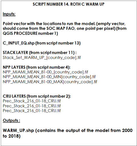
This script runs the spatial RothC model for the warm-up period (from 2001 to 2018). We will provide the script the target points (empty vector layer from Qgis procedure number 1), the Stack layer (from script number 11), the three NPP layers (from script number 5) and the three climate layers generated in script number 2. The output vector layer from script number 13 (Spin up phase) will also be needed.
rm(list=ls())
library(SoilR)
library(raster)
library(rgdal)
library(soilassessment)
working_dir<-setwd("C:/TRAINING_MATERIALS_GSOCseq_MAPS_28-09-2020")
#Open empty vector
Vector<-readOGR("INPUTS/TARGET_POINTS/target_points_sub.shp")
#Open Warm Up Stack
Stack_Set_warmup<- stack("INPUTS/STACK/Stack_Set_WARM_UP_AOI.tif")
# Open Result from SPIN UP PROCESS. A vector with 5 columns , one for each pool
Spin_up<-readOGR("OUTPUTS/1_SPIN_UP/SPIN_UP_County_AOI.shp")
Spin_up<-as.data.frame(Spin_up)

Spin_up<-as.data.frame(Spin_up)

# Open Precipitation , temperature, and EVapotranspiration file 20 anios x 12 = 240 layers x 3
# 216 layer stack
# CRU LAYERS
#PREC<-stack("INPUTS/CRU_LAYERS/Prec_Stack_216_01-18_CRU.tif")
#TEMP<-stack("INPUTS/CRU_LAYERS/Temp_Stack_216_01-18_CRU.tif")
#PET<-stack("INPUTS/CRU_LAYERS/PET_Stack_216_01-18_CRU.tif")

# TERRA CLIMATE LAYERS
PREC<-stack("INPUTS/TERRA_CLIME/Precipitation_2001-2021_Pergamino.tif")
TEMP<-stack("INPUTS/TERRA_CLIME/AverageTemperature_2001-2021_Pergamino.tif")*0.1
PET<-stack("INPUTS/TERRA_CLIME/PET_2001-2021_Pergamino.tif")*0.1

#Also check that the number of layers of DR and Land use are the same as the years of climate data.


#Open Mean NPP MIAMI 1981 - 2000


NPP<-raster("INPUTS/NPP/NPP_MIAMI_MEAN_81-00_AOI.tif")
NPP_MEAN_MIN<-raster("INPUTS/NPP/NPP_MIAMI_MEAN_81-00_AOI_MIN.tif")
NPP_MEAN_MAX<-raster("INPUTS/NPP/NPP_MIAMI_MEAN_81-00_AOI_MAX.tif")
#Open LU layer (year 2000).
LU_AOI<-raster("INPUTS/LAND_USE/ESA_Land_Cover_12clases_FAO_AOI.tif")
As we did in the “spin up” script, we will extract all variables to the target points and create an empty variable to save the results of the “warm up” process.
# Extract variables to points
Vector_points<-extract(Stack_Set_warmup,Vector,sp=TRUE)
Vector_points<-extract(TEMP,Vector_points,sp=TRUE)
Vector_points<-extract(PREC,Vector_points,sp=TRUE)
Vector_points<-extract(PET,Vector_points,sp=TRUE)
Vector_points<-extract(NPP,Vector_points,sp=TRUE)
Vector_points<-extract(NPP_MEAN_MIN,Vector_points,sp=TRUE)
Vector_points<-extract(NPP_MEAN_MAX,Vector_points,sp=TRUE)
WARM_UP<-Vector
Now, we will set some variables in order to run the model for the number of years according to those set for the climate layers. In this example we are running 18 years, but it can be run for less or more years.
# Warm Up number of years simulation
yearsSimulation<-dim(TEMP)[3]/12
clim_layers<-yearsSimulation*12
nppBand<-nlayers(Stack_Set_warmup)+clim_layers*3+2
firstClimLayer<-nlayers(Stack_Set_warmup)+2
nppBand_min<-nppBand+1
nppBand_max<-nppBand+2
nDR_beg<-(16+yearsSimulation)
nDR_end<-nDR_beg+(yearsSimulation-1)
Then we will set the variables in separate R variables:
# Extract the layers from the Vector
SOC_im<-Vector_points[[2]]
clay_im<-Vector_points[[3]]
LU_im<-Vector_points[[16]]
NPP_im<-Vector_points[[nppBand]]
NPP_im_MIN<-Vector_points[[nppBand_min]]
NPP_im_MAX<-Vector_points[[nppBand_max]]
We need to define the years of the “warm up” phase. Remember that we will run one year at a time with different pools of data for each year.
# Define Year
year=seq(1/12,1,by=1/12)
We will need to set the RothC function to be ready to be used in the “Warm Up” process.
###########function set up starts################
Roth_C<-function(Cinputs,years,DPMptf, RPMptf, BIOptf, HUMptf, FallIOM,Temp,Precip,Evp,Cov,Cov1,Cov2,soil.thick,SOC,clay,DR,bare1,LU)

{

# Paddy fields coefficent fPR = 0.4 if the target point is class = 13 , else fPR=1
# From Shirato and Yukozawa 2004

fPR=(LU == 13)*0.4 + (LU!=13)*1

#Temperature effects per month
fT=fT.RothC(Temp[,2])

#Moisture effects per month . Si se usa evapotranspiracion pE=1

fw1func<-function(P, E, S.Thick = 30, pClay = 32.0213, pE = 1, bare)
{

    M = P - E * pE
    Acc.TSMD = NULL
    for (i in 2:length(M)) {
    B = ifelse(bare[i] == FALSE, 1, 1.8)
     Max.TSMD = -(20 + 1.3 * pClay - 0.01 * (pClay^2)) * (S.Thick/23) * (1/B)
        Acc.TSMD[1] = ifelse(M[1] > 0, 0, M[1])
        if (Acc.TSMD[i - 1] + M[i] < 0) {
            Acc.TSMD[i] = Acc.TSMD[i - 1] + M[i]
        }
        else (Acc.TSMD[i] = 0)
        if (Acc.TSMD[i] <= Max.TSMD) {
            Acc.TSMD[i] = Max.TSMD
        }
    }
    b = ifelse(Acc.TSMD > 0.444 * Max.TSMD, 1, (0.2 + 0.8 * ((Max.TSMD -
        Acc.TSMD)/(Max.TSMD - 0.444 * Max.TSMD))))
    b<-clamp(b,lower=0.2)
    return(data.frame(b))
}


fW_2<- fw1func(P=(Precip[,2]), E=(Evp[,2]), S.Thick = soil.thick, pClay = clay, pE = 1, bare=bare1)$b

#Vegetation Cover effects  C1: No till Agriculture, C2: Conventional Agriculture, C3: Grasslands and Forests, C4 bareland and Urban

fC<-Cov2[,2]

# Set the factors frame for Model calculations

xi.frame=data.frame(years,rep(fT*fW_2*fC*fPR,length.out=length(years)))

# RUN THE MODEL from SoilR
#Loads the model Si pass=TRUE genera calcula el modelo aunque sea invalido.
#Model3_spin=RothCModel(t=years,C0=c(DPMptf, RPMptf, BIOptf, HUMptf, FallIOM),In=Cinputs,DR=DR,clay=clay,xi=xi.frame, pass=TRUE)
#Calculates stocks for each pool per month
#Ct3_spin=getC(Model3_spin)

# RUN THE MODEL from soilassesment

Model3_spin=carbonTurnover(tt=years,C0=c(DPMptf, RPMptf, BIOptf, HUMptf, FallIOM),In=Cinputs,Dr=DR,clay=clay,effcts=xi.frame, "euler")

Ct3_spin=Model3_spin[,2:6]

# Get the final pools of the time series

poolSize3_spin=as.numeric(tail(Ct3_spin,1))

return(poolSize3_spin)

}
##############funtion set up ends##########
Then, we will apply the function for each target point 18/20 times according to the number of years of the “warm up” process. We will also create empty variables called “Cinputs”,“Cinputs_min”, “Cinputs_max”,“NPP_M”,
"NPP_M_MIN","NPP_M_MAX".
Cinputs<-c()
Cinputs_min<-c()
Cinputs_max<-c()
NPP_M_MIN<-c()
NPP_M_MAX<-c()
NPP_M<-c()
# Iterates over the area of interest and over 18 years
###########for loop starts################
for (i in 1:(length(Vector_points))) {
At his step, the iteration over the number of years of the warm up process is started:
gt<-firstClimLayer
gp<-gt+clim_layers
gevp<-gp+clim_layers
for (w in 1:(dim(TEMP)[3]/12)) {
#print(c("year:",w))
# Extract the variables
Vect<-as.data.frame(Vector_points[i,])
Temp<-as.data.frame(t(Vect[gt:(gt+11)]))
Temp<-data.frame(Month=1:12, Temp=Temp[,1])
Precip<-as.data.frame(t(Vect[gp:(gp+11)]))
Precip<-data.frame(Month=1:12, Precip=Precip[,1])
Evp<-as.data.frame(t(Vect[gevp:(gevp+11)]))
Evp<-data.frame(Month=1:12, Evp=Evp[,1])
Cov<-as.data.frame(t(Vect[4:15]))
Cov1<-data.frame(Cov=Cov[,1])
Cov2<-data.frame(Month=1:12, Cov=Cov[,1])
DR_im<-as.data.frame(t(Vect[nDR_beg:nDR_end])) # DR one per year according to LU
DR_im<-data.frame(DR_im=DR_im[,1])
gt<-gt+12
gp<-gp+12
gevp<-gevp+12
This line will avoid running the model over points with unreliable values:
#Avoid calculus over Na values
if (any(is.na(Evp[,2])) | any(is.na(Temp[,2])) | any(is.na(SOC_im[i])) | any(is.na(clay_im[i])) | any(is.na(Spin_up[i,3]))  | any(is.na(NPP_im[i])) | any(is.na(Precip[,2]))  |  any(is.na(Cov2[,2]))  |  any(is.na(Cov1[,1]))  | any(is.na(DR_im[,1]))  | any(is.na(NPP_M[,1]))  |  (SOC_im[i]<0) | (clay_im[i]<0) | (Spin_up[i,3]<=0) ) {WARM_UP[i,2]<-0}else{
We will set the rest of the variables for each target point i and year w:
# Get the variables from the vector
soil.thick=30  #Soil thickness (organic layer topsoil), in cm
SOC<-SOC_im[i]      #Soil organic carbon in Mg/ha
clay<-clay_im[i]        #Percent clay %
DR<-DR_im[w,1]              # DPM/RPM (decomposable vs resistant plant material.)
bare1<-(Cov1>0.8)           # If the surface is bare or vegetated
NPP_81_00<-NPP_im[i]
NPP_81_00_MIN<-NPP_im_MIN[i]
NPP_81_00_MAX<-NPP_im_MAX[i]
We will calculate the NPP MIAMI value for each point and each year , and adjust the carbon inputs with the NPP values. The first Cinput value corresponds to the Cinput of equilibrium calculated in the Spin Up phase (Spin_up[i,3]).
# Cinputs
T<-mean(Temp[,2])
P<-sum(Precip[,2])
NPP_M[w]<-NPPmodel(P,T,"miami")*(1/100)*0.5
NPP_M[w]<-(LU_im[i]==2)*NPP_M[w]*0.53+ (LU_im[i]==4)*NPP_M[w]*0.88 + (LU_im[i]==3 | LU_im[i]==5 | LU_im[i]==6 | LU_im[i]==8)*NPP_M[w]*0.72
if (w==1) {Cinputs[w]<-(Spin_up[i,3]/NPP_81_00)*NPP_M[w]} else {Cinputs[w]<-(Cinputs[[w-1]]/ NPP_M[w-1]) * NPP_M[w]}
Then we will repeat the same code but this time changing the environmental variables to match the maximum and minimum values.
# Cinputs MIN
Tmin<-mean(Temp[,2]*1.02)
Pmin<-sum(Precip[,2]*0.95)
NPP_M_MIN[w]<-NPPmodel(Pmin,Tmin,"miami")*(1/100)*0.5
NPP_M_MIN[w]<-(LU_im[i]==2)*NPP_M_MIN[w]*0.53+ (LU_im[i]==4)*NPP_M_MIN[w]*0.88 + (LU_im[i]==3 | LU_im[i]==5 | LU_im[i]==6 | LU_im[i]==8)*NPP_M_MIN[w]*0.72
if (w==1) {Cinputs_min[w]<-(Spin_up[i,10]/NPP_81_00)*NPP_M_MIN[w]} else {Cinputs_min[w]<-(Cinputs_min[[w-1]]/ NPP_M_MIN[w-1]) * NPP_M_MIN[w]}
# Cinputs MAX
Tmax<-mean(Temp[,2]*0.98)
Pmax<-sum(Precip[,2]*1.05)
NPP_M_MAX[w]<-NPPmodel(Pmax,Tmax,"miami")*(1/100)*0.5
NPP_M_MAX[w]<-(LU_im[i]==2)*NPP_M_MAX[w]*0.53+ (LU_im[i]==4)*NPP_M_MAX[w]*0.88 + (LU_im[i]==3 | LU_im[i]==5 | LU_im[i]==6 | LU_im[i]==8)*NPP_M_MAX[w]*0.72
if (w==1) {Cinputs_max[w]<-(Spin_up[i,11]/NPP_81_00)*NPP_M_MAX[w]} else {Cinputs_max[w]<-(Cinputs_max[[w-1]]/ NPP_M_MAX[w-1]) * NPP_M_MAX[w]}
We will then run the RothC function for each point and each year. The first year we will use the equilibrium Cinputs, and the carbon pools obtained from the Spin Up phase. Then we will use the yearly adjusted Cinputs (using NPP) and the pools calculated from the previous iteration.
# Run the model for 2001-2018
if (w==1) {
f_wp<-Roth_C(Cinputs=Cinputs[1],years=year,DPMptf=Spin_up[i,5], RPMptf=Spin_up[i,6], BIOptf=Spin_up[i,7], HUMptf=Spin_up[i,8], FallIOM=Spin_up[i,9],Temp=Temp,Precip=Precip,Evp=Evp,Cov=Cov,Cov1=Cov1,Cov2=Cov2,soil.thick=soil.thick,SOC=SOC,clay=clay,DR=DR,bare1=bare1)
} else {
f_wp<-Roth_C(Cinputs=Cinputs[w],years=year,DPMptf=f_wp[1], RPMptf=f_wp[2], BIOptf=f_wp[3], HUMptf=f_wp[4], FallIOM=f_wp[5],Temp=Temp,Precip=Precip,Evp=Evp,Cov=Cov,Cov1=Cov1,Cov2=Cov2,soil.thick=soil.thick,SOC=SOC,clay=clay,DR=DR,bare1=bare1)
}
f_wp_t<-f_wp[1]+f_wp[2]+f_wp[3]+f_wp[4]+f_wp[5]
# Run the model for minimum values
if (w==1) {
f_wp_min<-Roth_C(Cinputs=Cinputs_min[1],years=years,DPMptf=Spin_up[i,13], RPMptf=Spin_up[i,14], BIOptf=Spin_up[i,15], HUMptf=Spin_up[i,16], FallIOM=Spin_up[i,17],Temp=Temp*1.02,Precip=Precip*0.95,Evp=Evp,Cov=Cov,Cov1=Cov1,Cov2=Cov2,soil.thick=soil.thick,SOC=SOC*0.8,clay=clay*0.9,DR=DR,bare1=bare1)
} else {
f_wp_min<-Roth_C(Cinputs=Cinputs_min[w],years=years,DPMptf=f_wp_min[1], RPMptf=f_wp_min[2], BIOptf=f_wp_min[3], HUMptf=f_wp_min[4], FallIOM=f_wp_min[5],Temp=Temp*1.02,Precip=Precip*0.95,Evp=Evp,Cov=Cov,Cov1=Cov1,Cov2=Cov2,soil.thick=soil.thick,SOC=SOC*0.8,clay=clay*0.9,DR=DR,bare1=bare1)
}
f_wp_t_min<-f_wp_min[1]+f_wp_min[2]+f_wp_min[3]+f_wp_min[4]+f_wp_min[5]
# Run the model for maximum values
if (w==1) {
f_wp_max<-Roth_C(Cinputs=Cinputs_max[1],years=years,DPMptf=Spin_up[i,19], RPMptf=Spin_up[i,20], BIOptf=Spin_up[i,21], HUMptf=Spin_up[i,22], FallIOM=Spin_up[i,23],Temp=Temp*0.98,Precip=Precip*1.05,Evp=Evp,Cov=Cov,Cov1=Cov1,Cov2=Cov2,soil.thick=soil.thick,SOC=SOC*1.2,clay=clay*1.1,DR=DR,bare1=bare1)
} else {
f_wp_max<-Roth_C(Cinputs=Cinputs_max[w],years=years,DPMptf=f_wp_max[1], RPMptf=f_wp_max[2], BIOptf=f_wp_max[3], HUMptf=f_wp_max[4], FallIOM=f_wp_max[5],Temp=Temp*0.98,Precip=Precip*1.05,Evp=Evp,Cov=Cov,Cov1=Cov1,Cov2=Cov2,soil.thick=soil.thick,SOC=SOC*1.2,clay=clay*1.1,DR=DR,bare1=bare1)
}
f_wp_t_max<-f_wp_max[1]+f_wp_max[2]+f_wp_max[3]+f_wp_max[4]+f_wp_max[5]
print(w)
print(c(i,SOC,Spin_up[i,3],NPP_81_00,NPP_M[w,1],Cinputs[w],f_wp_t,DR_im[w,1]))
}
}
We will save the results from the iteration of the last year to the empty vector. We will also calculate an average of all the Cinputs used in the warm up phase and save it. We will need this “CinputFOWARD” variable in the next phase (Forward) and script (script number 15).
if (is.na(mean(Cinputs))){ CinputFOWARD<-NA} else {
CinputFOWARD<-mean(Cinputs)
CinputFOWARD_min<-mean(Cinputs_min)
CinputFOWARD_max<-mean(Cinputs_max)
WARM_UP[i,2]<-SOC
WARM_UP[i,3]<-Cinputs[18]
WARM_UP[i,4]<-f_wp_t
WARM_UP[i,5]<-f_wp[1]
WARM_UP[i,6]<-f_wp[2]
WARM_UP[i,7]<-f_wp[3]
WARM_UP[i,8]<-f_wp[4]
WARM_UP[i,9]<-f_wp[5]
WARM_UP[i,10]<-CinputFOWARD
WARM_UP[i,11]<-f_wp_t_min
WARM_UP[i,12]<-f_wp_min[1]
WARM_UP[i,13]<-f_wp_min[2]
WARM_UP[i,14]<-f_wp_min[3]
WARM_UP[i,15]<-f_wp_min[4]
WARM_UP[i,16]<-f_wp_min[5]
WARM_UP[i,17]<-f_wp_t_max
WARM_UP[i,18]<-f_wp_max[1]
WARM_UP[i,19]<-f_wp_max[2]
WARM_UP[i,20]<-f_wp_max[3]
WARM_UP[i,21]<-f_wp_max[4]
WARM_UP[i,22]<-f_wp_max[5]
WARM_UP[i,23]<-CinputFOWARD_min
WARM_UP[i,24]<-CinputFOWARD_max
Cinputs<-c()
Cinputs_min<-c()
Cinputs_max<-c()
}
print(i)
}
###########for loop ends################
We will then run the last code block to change the names to the fields of the vector’s table.
colnames(WARM_UP@data)[2]="SOC_FAO"
colnames(WARM_UP@data)[3]="Cin_2018"
colnames(WARM_UP@data)[4]="SOC_2018"
colnames(WARM_UP@data)[5]="DPM_w_up"
colnames(WARM_UP@data)[6]="RPM_w_up"
colnames(WARM_UP@data)[7]="BIO_w_up"
colnames(WARM_UP@data)[8]="HUM_w_up"
colnames(WARM_UP@data)[9]="IOM_w_up"
colnames(WARM_UP@data)[10]="Cin_mean"
colnames(WARM_UP@data)[11]="SOC_18min"
colnames(WARM_UP@data)[12]="DPM_w_min"
colnames(WARM_UP@data)[13]="RPM_w_min"
colnames(WARM_UP@data)[14]="BIO_w_min"
colnames(WARM_UP@data)[15]="HUM_w_min"
colnames(WARM_UP@data)[16]="IOM_w_min"
colnames(WARM_UP@data)[17]="SOC_18max"
colnames(WARM_UP@data)[18]="DPM_w_max"
colnames(WARM_UP@data)[19]="RPM_w_max"
colnames(WARM_UP@data)[20]="BIO_w_max"
colnames(WARM_UP@data)[21]="HUM_w_max"
colnames(WARM_UP@data)[22]="IOM_w_max"
colnames(WARM_UP@data)[23]="Cin_min"
colnames(WARM_UP@data)[24]="Cin_max"
Finally, we will have to save the output vector and the name of that vector.
 # SAVE the Points (shapefile)
writeOGR(WARM_UP,".", "OUTPUTS/2_WARM_UP/WARM_UP_County_AOI", driver="ESRI Shapefile")
10.3.2 Script Number 14B. “ROTH_C_WARM_UP_v4.R” Land use change simulation
This script is provided as an alternative in the case that yearly land use layers are available as input for the the warm up phase to account form land use change.
#12/11/2020

# SPATIAL SOIL R  for VECTORS

#   ROTH C phase 3: WARM UP

# MSc Ing Agr Luciano E Di Paolo
# Dr Ing Agr Guillermo E Peralta
###################################
# SOilR from Sierra, C.A., M. Mueller, S.E. Trumbore (2012).
#Models of soil organic matter decomposition: the SoilR package, version 1.0 Geoscientific Model Development, 5(4),
#1045--1060. URL http://www.geosci-model-dev.net/5/1045/2012/gmd-5-1045-2012.html.
#####################################

rm(list=ls())

library(SoilR)
library(raster)
library(rgdal)
library(soilassessment)

working_dir<-setwd("C:/TRAINING_MATERIALS_GSOCseq_MAPS_12-11-2020")

#Open empty vector

Vector<-readOGR("INPUTS/TARGET_POINTS/target_points_sub.shp")

#Open Warm Up Stack

Stack_Set_warmup<- stack("INPUTS/STACK/Stack_Set_WARM_UP_AOI.tif")

# Open Result from SPIN UP PROCESS. A vector with 5 columns , one for each pool

Spin_up<-readOGR("D:/TRAINING_MATERIALS_GSOCseq_MAPS_12-11-2020/OUTPUTS/1_SPIN_UP/SPIN_UP_County_AOI.shp")
Spin_up<-as.data.frame(Spin_up)

# Open Precipitation , temperature, and EVapotranspiration file 20 anios x 12 = 240 layers x 3
# 216 layer stack
# CRU LAYERS
#PREC<-stack("INPUTS/CRU_LAYERS/Prec_Stack_216_01-18_CRU.tif")
#TEMP<-stack("INPUTS/CRU_LAYERS/Temp_Stack_216_01-18_CRU.tif")
#PET<-stack("INPUTS/CRU_LAYERS/PET_Stack_216_01-18_CRU.tif")

# TERRA CLIMATE LAYERS
PREC<-stack("INPUTS/TERRA_CLIME/Precipitation_2001-2021_Pergamino.tif")
TEMP<-stack("INPUTS/TERRA_CLIME/AverageTemperature_2001-2021_Pergamino.tif")*0.1
PET<-stack("INPUTS/TERRA_CLIME/PET_2001-2021_Pergamino.tif")*0.1

#Also check that the number of layers of DR and Land use are the same as the years of climate data.


#Open Mean NPP MIAMI 1981 - 2000
NPP<-raster("INPUTS/NPP/NPP_MIAMI_MEAN_81-00_AOI.tif")

NPP_MEAN_MIN<-raster("INPUTS/NPP/NPP_MIAMI_MEAN_81-00_AOI_MIN.tif")

NPP_MEAN_MAX<-raster("INPUTS/NPP/NPP_MIAMI_MEAN_81-00_AOI_MAX.tif")

#Open LU layer (year 2000).

#LU_AOI<-raster("INPUTS/LAND_USE/ESA_Land_Cover_12clases_FAO_AOI.tif")
LU_AOI<-Stack_Set_warmup[[15]]# LU 2001

#Apply NPP coeficientes
NPP<-(LU_AOI==2 | LU_AOI==12 | LU_AOI==13)*NPP*0.53+ (LU_AOI==4)*NPP*0.88 + (LU_AOI==3 | LU_AOI==5 | LU_AOI==6 | LU_AOI==8)*NPP*0.72
NPP_MEAN_MIN<-(LU_AOI==2 | LU_AOI==12 | LU_AOI==13)*NPP_MEAN_MIN*0.53+ (LU_AOI==4)*NPP_MEAN_MIN*0.88 + (LU_AOI==3 | LU_AOI==5 | LU_AOI==6 | LU_AOI==8)*NPP_MEAN_MIN*0.72
NPP_MEAN_MAX<-(LU_AOI==2 | LU_AOI==12 | LU_AOI==13)*NPP_MEAN_MAX*0.53+ (LU_AOI==4)*NPP_MEAN_MAX*0.88 + (LU_AOI==3 | LU_AOI==5 | LU_AOI==6 | LU_AOI==8)*NPP_MEAN_MAX*0.72


# Extract variables to points

Vector_points<-extract(Stack_Set_warmup,Vector,sp=TRUE)
Vector_points<-extract(TEMP,Vector_points,sp=TRUE)
Vector_points<-extract(PREC,Vector_points,sp=TRUE)
Vector_points<-extract(PET,Vector_points,sp=TRUE)
Vector_points<-extract(NPP,Vector_points,sp=TRUE)
Vector_points<-extract(NPP_MEAN_MIN,Vector_points,sp=TRUE)
Vector_points<-extract(NPP_MEAN_MAX,Vector_points,sp=TRUE)

WARM_UP<-Vector

#use only for backup

#WARM_UP<-readOGR("WARM_UP_County_AOI3_97.shp")

# Warm Up number of years simulation

yearsSimulation<-dim(TEMP)[3]/12

clim_layers<-yearsSimulation*12

nppBand<-nlayers(Stack_Set_warmup)+clim_layers*3+2

firstClimLayer<-nlayers(Stack_Set_warmup)+2

nppBand_min<-nppBand+1

nppBand_max<-nppBand+2

nDR_beg<-(16+yearsSimulation)
nDR_end<-nDR_beg+(yearsSimulation-1)

nLU_beg<-16
nLU_end<-nLU_beg+(yearsSimulation-1)

# Extract the layers from the Vector

SOC_im<-Vector_points[[2]]

clay_im<-Vector_points[[3]]

#LU_im<-Vector_points[[16:34]]

NPP_im<-Vector_points[[nppBand]]

NPP_im_MIN<-Vector_points[[nppBand_min]]

NPP_im_MAX<-Vector_points[[nppBand_max]]

# Define Years

years=seq(1/12,1,by=1/12)


# ROTH C MODEL FUNCTION .

###########function set up starts################
Roth_C<-function(Cinputs,years,DPMptf, RPMptf, BIOptf, HUMptf, FallIOM,Temp,Precip,Evp,Cov,Cov1,Cov2,soil.thick,SOC,clay,DR,bare1,LU)

{

# Paddy fields coefficent fPR = 0.4 if the target point is class = 13 , else fPR=1
# From Shirato and Yukozawa 2004

fPR=(LU == 13)*0.4 + (LU!=13)*1

#Temperature effects per month
fT=fT.RothC(Temp[,2])

#Moisture effects per month . Si se usa evapotranspiracion pE=1

fw1func<-function(P, E, S.Thick = 30, pClay = 32.0213, pE = 1, bare)
{

    M = P - E * pE
    Acc.TSMD = NULL
    for (i in 2:length(M)) {
    B = ifelse(bare[i] == FALSE, 1, 1.8)
     Max.TSMD = -(20 + 1.3 * pClay - 0.01 * (pClay^2)) * (S.Thick/23) * (1/B)
        Acc.TSMD[1] = ifelse(M[1] > 0, 0, M[1])
        if (Acc.TSMD[i - 1] + M[i] < 0) {
            Acc.TSMD[i] = Acc.TSMD[i - 1] + M[i]
        }
        else (Acc.TSMD[i] = 0)
        if (Acc.TSMD[i] <= Max.TSMD) {
            Acc.TSMD[i] = Max.TSMD
        }
    }
    b = ifelse(Acc.TSMD > 0.444 * Max.TSMD, 1, (0.2 + 0.8 * ((Max.TSMD -
        Acc.TSMD)/(Max.TSMD - 0.444 * Max.TSMD))))
    b<-clamp(b,lower=0.2)
    return(data.frame(b))
}


fW_2<- fw1func(P=(Precip[,2]), E=(Evp[,2]), S.Thick = soil.thick, pClay = clay, pE = 1, bare=bare1)$b

#Vegetation Cover effects  C1: No till Agriculture, C2: Conventional Agriculture, C3: Grasslands and Forests, C4 bareland and Urban

fC<-Cov2[,2]

# Set the factors frame for Model calculations

xi.frame=data.frame(years,rep(fT*fW_2*fC*fPR,length.out=length(years)))

# RUN THE MODEL from SoilR
#Loads the model Si pass=TRUE genera calcula el modelo aunque sea invalido.
#Model3_spin=RothCModel(t=years,C0=c(DPMptf, RPMptf, BIOptf, HUMptf, FallIOM),In=Cinputs,DR=DR,clay=clay,xi=xi.frame, pass=TRUE)
#Calculates stocks for each pool per month
#Ct3_spin=getC(Model3_spin)

# RUN THE MODEL from soilassesment

Model3_spin=carbonTurnover(tt=years,C0=c(DPMptf, RPMptf, BIOptf, HUMptf, FallIOM),In=Cinputs,Dr=DR,clay=clay,effcts=xi.frame, "euler")

Ct3_spin=Model3_spin[,2:6]

# Get the final pools of the time series

poolSize3_spin=as.numeric(tail(Ct3_spin,1))

return(poolSize3_spin)

}
##############funtion set up ends##########

# Iterates over the area of interest and over 18 years

Cinputs<-c()
Cinputs_min<-c()
Cinputs_max<-c()
NPP_M_MIN<-c()
NPP_M_MAX<-c()
NPP_M<-c()

############for loop starts################
for (i in 1:(length(Vector_points))) {

gt<-firstClimLayer
gp<-gt+clim_layers
gevp<-gp+clim_layers

for (w in 1:(dim(TEMP)[3]/12)) {

print(c("year:",w))
# Extract the variables

Vect<-as.data.frame(Vector_points[i,])

Temp<-as.data.frame(t(Vect[gt:(gt+11)]))
Temp<-data.frame(Month=1:12, Temp=Temp[,1])

Precip<-as.data.frame(t(Vect[gp:(gp+11)]))
Precip<-data.frame(Month=1:12, Precip=Precip[,1])

Evp<-as.data.frame(t(Vect[gevp:(gevp+11)]))
Evp<-data.frame(Month=1:12, Evp=Evp[,1])

Cov<-as.data.frame(t(Vect[4:15]))
Cov1<-data.frame(Cov=Cov[,1])
Cov2<-data.frame(Month=1:12, Cov=Cov[,1])

DR_im<-as.data.frame(t(Vect[nDR_beg:nDR_end])) # DR one per year according to LU
DR_im<-data.frame(DR_im=DR_im[,1])

LU_im<-as.data.frame(t(Vect[nLU_beg:nLU_end])) # DR one per year according to LU
LU_im<-data.frame(LU_im=LU_im[,1])

gt<-gt+12
gp<-gp+12
gevp<-gevp+12

#Avoid calculus over Na values

if (any(is.na(Evp[,2])) | any(is.na(Temp[,2])) | any(is.na(SOC_im[i])) | any(is.na(clay_im[i])) | any(is.na(Spin_up[i,3]))  | any(is.na(NPP_im[i])) | any(is.na(Precip[,2]))  |  any(is.na(Cov2[,2]))  |  any(is.na(Cov1[,1]))  | any(is.na(DR_im[,1]))    |  (SOC_im[i]<0) | (clay_im[i]<0) | (Spin_up[i,3]<=0) ) {WARM_UP[i,2]<-0}else{

# Get the variables from the vector

soil.thick=30  #Soil thickness (organic layer topsoil), in cm
SOC<-SOC_im[i]      #Soil organic carbon in Mg/ha
clay<-clay_im[i]        #Percent clay %

DR<-DR_im[w,1]              # DPM/RPM (decomplosable vs resistant plant material.)
LU<-LU_im[w,1]
bare1<-(Cov1>0.8)           # If the surface is bare or vegetated
NPP_81_00<-NPP_im[i]
NPP_81_00_MIN<-NPP_im_MIN[i]
NPP_81_00_MAX<-NPP_im_MAX[i]

# PHASE 2  : WARM UP .  years (w)

# Cinputs
T<-mean(Temp[,2])
P<-sum(Precip[,2])
NPP_M[w]<-NPPmodel(P,T,"miami")*(1/100)*0.5
NPP_M[w]<-(LU==2 | LU==12 | LU==13)*NPP_M[w]*0.53+ (LU==4)*NPP_M[w]*0.88 + (LU==3 | LU==5 | LU==6 | LU==8)*NPP_M[w]*0.72

if (w==1) {Cinputs[w]<-(Spin_up[i,3]/NPP_81_00)*NPP_M[w]} else {Cinputs[w]<-(Cinputs[[w-1]]/ NPP_M[w-1]) * NPP_M[w]}

# Cinputs MIN

Tmin<-mean(Temp[,2]*1.02)
Pmin<-sum(Precip[,2]*0.95)
NPP_M_MIN[w]<-NPPmodel(Pmin,Tmin,"miami")*(1/100)*0.5
NPP_M_MIN[w]<-(LU==2 | LU==12 | LU==13)*NPP_M_MIN[w]*0.53+ (LU==4)*NPP_M_MIN[w]*0.88 + (LU==3 | LU==5 | LU==6 | LU==8)*NPP_M_MIN[w]*0.72

if (w==1) {Cinputs_min[w]<-(Spin_up[i,10]/NPP_81_00)*NPP_M_MIN[w]} else {Cinputs_min[w]<-(Cinputs_min[[w-1]]/ NPP_M_MIN[w-1]) * NPP_M_MIN[w]}

# Cinputs MAX

Tmax<-mean(Temp[,2]*0.98)
Pmax<-sum(Precip[,2]*1.05)
NPP_M_MAX[w]<-NPPmodel(Pmax,Tmax,"miami")*(1/100)*0.5
NPP_M_MAX[w]<-(LU==2 | LU==12 | LU==13)*NPP_M_MAX[w]*0.53+ (LU==4)*NPP_M_MAX[w]*0.88 + (LU==3 | LU==5 | LU==6 | LU==8)*NPP_M_MAX[w]*0.72

if (w==1) {Cinputs_max[w]<-(Spin_up[i,11]/NPP_81_00)*NPP_M_MAX[w]} else {Cinputs_max[w]<-(Cinputs_max[[w-1]]/ NPP_M_MAX[w-1]) * NPP_M_MAX[w]}

# Run the model for 2001-2018

if (w==1) {
f_wp<-Roth_C(Cinputs=Cinputs[1],years=years,DPMptf=Spin_up[i,5], RPMptf=Spin_up[i,6], BIOptf=Spin_up[i,7], HUMptf=Spin_up[i,8], FallIOM=Spin_up[i,9],Temp=Temp,Precip=Precip,Evp=Evp,Cov=Cov,Cov1=Cov1,Cov2=Cov2,soil.thick=soil.thick,SOC=SOC,clay=clay,DR=DR,bare1=bare1,LU=LU)
} else {
f_wp<-Roth_C(Cinputs=Cinputs[w],years=years,DPMptf=f_wp[1], RPMptf=f_wp[2], BIOptf=f_wp[3], HUMptf=f_wp[4], FallIOM=f_wp[5],Temp=Temp,Precip=Precip,Evp=Evp,Cov=Cov,Cov1=Cov1,Cov2=Cov2,soil.thick=soil.thick,SOC=SOC,clay=clay,DR=DR,bare1=bare1,LU=LU)
}

f_wp_t<-f_wp[1]+f_wp[2]+f_wp[3]+f_wp[4]+f_wp[5]

# Run the model for minimum values

if (w==1) {
f_wp_min<-Roth_C(Cinputs=Cinputs_min[1],years=years,DPMptf=Spin_up[i,13], RPMptf=Spin_up[i,14], BIOptf=Spin_up[i,15], HUMptf=Spin_up[i,16], FallIOM=Spin_up[i,17],Temp=Temp*1.02,Precip=Precip*0.95,Evp=Evp,Cov=Cov,Cov1=Cov1,Cov2=Cov2,soil.thick=soil.thick,SOC=SOC*0.8,clay=clay*0.9,DR=DR,bare1=bare1,LU=LU)
} else {
f_wp_min<-Roth_C(Cinputs=Cinputs_min[w],years=years,DPMptf=f_wp_min[1], RPMptf=f_wp_min[2], BIOptf=f_wp_min[3], HUMptf=f_wp_min[4], FallIOM=f_wp_min[5],Temp=Temp*1.02,Precip=Precip*0.95,Evp=Evp,Cov=Cov,Cov1=Cov1,Cov2=Cov2,soil.thick=soil.thick,SOC=SOC*0.8,clay=clay*0.9,DR=DR,bare1=bare1,LU=LU)
}

f_wp_t_min<-f_wp_min[1]+f_wp_min[2]+f_wp_min[3]+f_wp_min[4]+f_wp_min[5]

# Run the model for maximum values

if (w==1) {
f_wp_max<-Roth_C(Cinputs=Cinputs_max[1],years=years,DPMptf=Spin_up[i,19], RPMptf=Spin_up[i,20], BIOptf=Spin_up[i,21], HUMptf=Spin_up[i,22], FallIOM=Spin_up[i,23],Temp=Temp*0.98,Precip=Precip*1.05,Evp=Evp,Cov=Cov,Cov1=Cov1,Cov2=Cov2,soil.thick=soil.thick,SOC=SOC*1.2,clay=clay*1.1,DR=DR,bare1=bare1,LU=LU)
} else {
f_wp_max<-Roth_C(Cinputs=Cinputs_max[w],years=years,DPMptf=f_wp_max[1], RPMptf=f_wp_max[2], BIOptf=f_wp_max[3], HUMptf=f_wp_max[4], FallIOM=f_wp_max[5],Temp=Temp*0.98,Precip=Precip*1.05,Evp=Evp,Cov=Cov,Cov1=Cov1,Cov2=Cov2,soil.thick=soil.thick,SOC=SOC*1.2,clay=clay*1.1,DR=DR,bare1=bare1,LU=LU)
}

f_wp_t_max<-f_wp_max[1]+f_wp_max[2]+f_wp_max[3]+f_wp_max[4]+f_wp_max[5]

print(w)
#print(c(i,SOC,Spin_up[i,3],NPP_81_00,Cinputs[w],f_wp_t))
print(c(NPP_M[w],Cinputs[w]))
}
}
if (is.na(mean(Cinputs))){ CinputFOWARD<-NA} else {

CinputFOWARD<-mean(Cinputs)

CinputFOWARD_min<-mean(Cinputs_min)

CinputFOWARD_max<-mean(Cinputs_max)

WARM_UP[i,2]<-SOC
WARM_UP[i,3]<-Cinputs[18]
WARM_UP[i,4]<-f_wp_t
WARM_UP[i,5]<-f_wp[1]
WARM_UP[i,6]<-f_wp[2]
WARM_UP[i,7]<-f_wp[3]
WARM_UP[i,8]<-f_wp[4]
WARM_UP[i,9]<-f_wp[5]
WARM_UP[i,10]<-CinputFOWARD
WARM_UP[i,11]<-f_wp_t_min
WARM_UP[i,12]<-f_wp_min[1]
WARM_UP[i,13]<-f_wp_min[2]
WARM_UP[i,14]<-f_wp_min[3]
WARM_UP[i,15]<-f_wp_min[4]
WARM_UP[i,16]<-f_wp_min[5]
WARM_UP[i,17]<-f_wp_t_max
WARM_UP[i,18]<-f_wp_max[1]
WARM_UP[i,19]<-f_wp_max[2]
WARM_UP[i,20]<-f_wp_max[3]
WARM_UP[i,21]<-f_wp_max[4]
WARM_UP[i,22]<-f_wp_max[5]
WARM_UP[i,23]<-CinputFOWARD_min
WARM_UP[i,24]<-CinputFOWARD_max

Cinputs<-c()
Cinputs_min<-c()
Cinputs_max<-c()
}
print(i)
}

################for loop ends#############

colnames(WARM_UP@data)[2]="SOC_FAO"
colnames(WARM_UP@data)[3]="Cin_t0"
colnames(WARM_UP@data)[4]="SOC_t0"
colnames(WARM_UP@data)[5]="DPM_w_up"
colnames(WARM_UP@data)[6]="RPM_w_up"
colnames(WARM_UP@data)[7]="BIO_w_up"
colnames(WARM_UP@data)[8]="HUM_w_up"
colnames(WARM_UP@data)[9]="IOM_w_up"
colnames(WARM_UP@data)[10]="Cin_mean"
colnames(WARM_UP@data)[11]="SOC_t0min"
colnames(WARM_UP@data)[12]="DPM_w_min"
colnames(WARM_UP@data)[13]="RPM_w_min"
colnames(WARM_UP@data)[14]="BIO_w_min"
colnames(WARM_UP@data)[15]="HUM_w_min"
colnames(WARM_UP@data)[16]="IOM_w_min"
colnames(WARM_UP@data)[17]="SOC_t0max"
colnames(WARM_UP@data)[18]="DPM_w_max"
colnames(WARM_UP@data)[19]="RPM_w_max"
colnames(WARM_UP@data)[20]="BIO_w_max"
colnames(WARM_UP@data)[21]="HUM_w_max"
colnames(WARM_UP@data)[22]="IOM_w_max"
colnames(WARM_UP@data)[23]="Cin_min"
colnames(WARM_UP@data)[24]="Cin_max"


# SAVE the Points (shapefile)
setwd("C:/TRAINING_MATERIALS_GSOCseq_MAPS_12-11-2020/OUTPUTS/2_WARM_UP")
writeOGR(WARM_UP,".", "WARM_UP_County_AOI_LUsim", driver="ESRI Shapefile",overwrite=TRUE)
10.4 Forward phase: Script Number 15. “ROTH_C_forward_v2.R”
Script number 15 implements the third modeling phase (“forward” phase). We will need to load the stack of layers generated in script number 12 and the target points. We will also need to load the output vector of the phase 2 (“warm up”) as an input. This script will run the Roth C model for 20 years, projecting SOC stocks for the 2020-2040 period under different management scenarios (“BAU” scenario and the three SSM scenarios: low, medium and high input carbon). C inputs will vary according to the SSM scenarios. Standard default values of 5-10-20% increase in C inputs are defined for the three SSM scenarios (low, medium, high, respectively). Users can modify these inputs based on local expertise and available information, and generate alternative maps using this data. The final outputs will be the final SOC stocks after 20 years for the different scenarios. This information will be saved to a shapefile.
Table 10.3 Script Number 15. forward phase. Inputs and Outputs
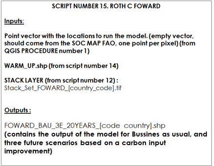
The ‘Forward’ modeling phase requires (as in the previous phases) the target points (generated from the Qgis procedure number 1), the stack of layers (from script number 12), and the output vector from the previous phase (warm up). We will need to load the R packages, the target points, the stack for this phase (Stack_Set_forward_[country_code].tif), and vector from the ‘Warm up’ phase (WARM_UP.shp).
rm(list=ls())
library(SoilR)
library(raster)
library(rgdal)
library(soilassessment)
WD_OUT<-("C:/TRAINING_MATERIALS_GSOCseq_MAPS_28-09-2020/OUTPUTS/3_FOWARD")
working_dir<-setwd("C:/TRAINING_MATERIALS_GSOCseq_MAPS_28-09-2020")
# OPEN THE VECTOR OF POINTS
Vector<-readOGR("INPUTS/TARGET_POINTS/target_points_sub.shp")
# OPEN THE RESULT VECTOR FROM THE WARM UP PROCESS
WARM_UP<-readOGR("OUTPUTS/2_WARM_UP/WARM_UP_County_AOI.shp")
# OPEN THE STACK WITH THE VARIABLES FOR THE FOWARD PROCESS
Stack_Set_1<- stack("INPUTS/STACK/Stack_Set_FOWARD.tif")
We can set the SSM carbon input increment of each land use class.
# Set the increase in Carbon input for each land use and each scenario
#Crops and Crop trees
Low_Crops<-1.05
Med_Crops<-1.10
High_Crops<-1.2
#Shrublands, Grasslands , Herbaceous vegetation flooded & Sparse Vegetation
Low_Grass<-1.05
Med_Grass<-1.10
High_Grass<-1.2
#Forest
Low_Forest<-1.05
Med_Forest<-1.10
High_Forest<-1.2
#Paddy Fields
Low_PaddyFields<-1.05
Med_PaddyFields<-1.10
High_PaddyFields<-1.2
Next, we will extract the variables contained in the stack to the target points.
# extract variables to points
Variables<-extract(Stack_Set_1,Vector,sp=TRUE)
Then we will create a variable to save the results from the simulations.
# Creates an empty vector
FOWARD<-Vector
We will extract some of the variables needed in the model to individual variables .
# Extract the layers from the Vector
SOC_im<-WARM_UP[[4]]
clay_im<-Variables[[3]]
Cinputs_im<-WARM_UP[[10]]
DR_im<-Variables[[40]]
LU_im<-Variables[[41]]
Next, we will define the number of years for the modeling runs.
# Define the years to run the model
years=seq(1/12,20,by=1/12)
Then, we will set the RothC function as we did for the previous modeling phases.
#############function set up starts###############
Roth_C<-function(Cinputs,years,DPMptf, RPMptf, BIOptf, HUMptf, FallIOM,Temp,Precip,Evp,Cov,Cov1,Cov2,soil.thick,SOC,clay,DR,bare1,LU)
{
# Paddy Fields coefficent fPR = 0.4 if the target point is class = 13 , else fPR=1
# From Shirato and Yukozawa 2004

fPR=(LU == 13)*0.4 + (LU!=13)*1

#Temperature effects per month
fT=fT.RothC(Temp[,2])

#Moisture effects per month .

fw1func<-function(P, E, S.Thick = 30, pClay = 32.0213, pE = 1, bare)
{

    M = P - E * pE
    Acc.TSMD = NULL
    for (i in 2:length(M)) {
    B = ifelse(bare[i] == FALSE, 1, 1.8)
     Max.TSMD = -(20 + 1.3 * pClay - 0.01 * (pClay^2)) * (S.Thick/23) * (1/B)
        Acc.TSMD[1] = ifelse(M[1] > 0, 0, M[1])
        if (Acc.TSMD[i - 1] + M[i] < 0) {
            Acc.TSMD[i] = Acc.TSMD[i - 1] + M[i]
        }
        else (Acc.TSMD[i] = 0)
        if (Acc.TSMD[i] <= Max.TSMD) {
            Acc.TSMD[i] = Max.TSMD
        }
    }
    b = ifelse(Acc.TSMD > 0.444 * Max.TSMD, 1, (0.2 + 0.8 * ((Max.TSMD -
        Acc.TSMD)/(Max.TSMD - 0.444 * Max.TSMD))))
    b<-clamp(b,lower=0.2)
    return(data.frame(b))
}

fW_2<- fw1func(P=(Precip[,2]), E=(Evp[,2]), S.Thick = soil.thick, pClay = clay, pE = 1, bare=bare1)$b

#Vegetation Cover effects

fC<-Cov2[,2]

# Set the factors frame for Model calculations

xi.frame=data.frame(years,rep(fT*fW_2*fC*fPR,length.out=length(years)))

# RUN THE MODEL from SoilR
#Loads the model
#Model3_spin=RothCModel(t=years,C0=c(DPMptf[[1]], RPMptf[[1]], BIOptf[[1]], HUMptf[[1]], FallIOM[[1]]),In=Cinputs,DR=DR,clay=clay,xi=xi.frame, pass=TRUE)
#Ct3_spin=getC(Model3_spin)

# RUN THE MODEL from soilassesment

Model3_spin=carbonTurnover(tt=years,C0=c(DPMptf[[1]], RPMptf[[1]], BIOptf[[1]], HUMptf[[1]], FallIOM[[1]]),In=Cinputs,Dr=DR,clay=clay,effcts=xi.frame, "euler")

Ct3_spin=Model3_spin[,2:6]

# Get the final pools of the time series

poolSize3_spin=as.numeric(tail(Ct3_spin,1))

return(poolSize3_spin)
}
################function set up ends#############
Then we can iterate over the vector variable, running the model for each target point.
# Iterates over the area of interest
##################for loop starts###############
for (i in 1:dim(Variables)[1]) {
# Extract the variables
Vect<-as.data.frame(Variables[i,])
Temp<-as.data.frame(t(Vect[4:15]))
Temp<-data.frame(Month=1:12, Temp=Temp[,1])
Precip<-as.data.frame(t(Vect[16:27]))
Precip<-data.frame(Month=1:12, Precip=Precip[,1])
Evp<-as.data.frame(t(Vect[28:39]))
Evp<-data.frame(Month=1:12, Evp=Evp[,1])
Cov<-as.data.frame(t(Vect[42:53]))
Cov1<-data.frame(Cov=Cov[,1])
Cov2<-data.frame(Month=1:12, Cov=Cov[,1])
#Avoid calculus over Na values
if (any(is.na(Evp[,2])) | any(is.na(Temp[,2])) | any(is.na(SOC_im[i])) | any(is.na(clay_im[i])) | any(is.na(Precip[,2]))  |  any(is.na(Cov2[,2]))  |  any(is.na(Cov1[,1])) | any(is.na(Cinputs_im[i])) | any(is.na(DR_im[i])) | (Cinputs_im[i]<0) |  (SOC_im[i]<0) | (clay_im[i]<0) ) {FOWARD[i,2]<-0}else{
# Set the variables from the images
soil.thick=30  #Soil thickness (organic layer topsoil), in cm
SOC<-SOC_im[i]      #Soil organic carbon in Mg/ha
clay<-clay_im[i]        #Percent clay %
Cinputs<-Cinputs_im[i]    #Annual C inputs to soil in Mg/ha/yr
DR<-DR_im[i]              # DPM/RPM (decomplosable vs resistant plant material.)
bare1<-(Cov1>0.8)           # If the surface is bare or vegetated
LU<-LU_im[i]
Now we can run the model for the business as usual (BAU) scenario. The “f_bau_t” variable will save the result of the model in each iteration.
# Final calculation of SOC  20 years in the future  (Business as usual)

f_bau<-Roth_C(Cinputs=Cinputs,years=years,DPMptf=WARM_UP[i,5], RPMptf=WARM_UP[i,6], BIOptf=WARM_UP[i,7], HUMptf=WARM_UP[i,8], FallIOM=WARM_UP[i,9],Temp=Temp,Precip=Precip,Evp=Evp,Cov=Cov,Cov1=Cov1,Cov2=Cov2,soil.thick=soil.thick,SOC=SOC,clay=clay,DR=DR,bare1=bare1,LU=LU)
f_bau_t<-f_bau[1]+f_bau[2]+f_bau[3]+f_bau[4]+f_bau[5]

#Unc BAU minimum
Cinputs_min<-WARM_UP@data[i,23]
Cinputs_max<-WARM_UP@data[i,24]
SOC_t0_min<-WARM_UP@data[i,11]
SOC_t0_max<-WARM_UP@data[i,17]

f_bau_min<-Roth_C(Cinputs=Cinputs_min,years=years,DPMptf=WARM_UP[i,12], RPMptf=WARM_UP[i,13], BIOptf=WARM_UP[i,14], HUMptf=WARM_UP[i,15], FallIOM=WARM_UP[i,16],Temp=Temp*1.02,Precip=Precip*0.95,Evp=Evp,Cov=Cov,Cov1=Cov1,Cov2=Cov2,soil.thick=soil.thick,SOC=SOC*0.8,clay=clay*0.9,DR=DR,bare1=bare1,LU=LU)
f_bau_t_min<-f_bau_min[1]+f_bau_min[2]+f_bau_min[3]+f_bau_min[4]+f_bau_min[5]

#Unc BAU maximum

f_bau_max<-Roth_C(Cinputs=Cinputs_max,years=years,DPMptf=WARM_UP[i,18], RPMptf=WARM_UP[i,19], BIOptf=WARM_UP[i,20], HUMptf=WARM_UP[i,21], FallIOM=WARM_UP[i,22],Temp=Temp*0.98,Precip=Precip*1.05,Evp=Evp,Cov=Cov,Cov1=Cov1,Cov2=Cov2,soil.thick=soil.thick,SOC=SOC*1.2,clay=clay*1.1,DR=DR,bare1=bare1,LU=LU)
f_bau_t_max<-f_bau_max[1]+f_bau_max[2]+f_bau_max[3]+f_bau_max[4]+f_bau_max[5]

# Crops and Tree crops
if (LU==2 | LU==12){
f_low<-Roth_C(Cinputs=(Cinputs*Low_Crops),years=years,DPMptf=WARM_UP[i,5], RPMptf=WARM_UP[i,6], BIOptf=WARM_UP[i,7], HUMptf=WARM_UP[i,8], FallIOM=WARM_UP[i,9],Temp=Temp,Precip=Precip,Evp=Evp,Cov=Cov,Cov1=Cov1,Cov2=Cov2,soil.thick=soil.thick,SOC=SOC,clay=clay,DR=DR,bare1=bare1,LU=LU)
f_low_t<-f_low[1]+f_low[2]+f_low[3]+f_low[4]+f_low[5]

f_med<-Roth_C(Cinputs=(Cinputs*Med_Crops),years=years,DPMptf=WARM_UP[i,5], RPMptf=WARM_UP[i,6], BIOptf=WARM_UP[i,7], HUMptf=WARM_UP[i,8], FallIOM=WARM_UP[i,9],Temp=Temp,Precip=Precip,Evp=Evp,Cov=Cov,Cov1=Cov1,Cov2=Cov2,soil.thick=soil.thick,SOC=SOC,clay=clay,DR=DR,bare1=bare1,LU=LU)
f_med_t<-f_med[1]+f_med[2]+f_med[3]+f_med[4]+f_med[5]

f_high<-Roth_C(Cinputs=(Cinputs*High_Crops),years=years,DPMptf=WARM_UP[i,5], RPMptf=WARM_UP[i,6], BIOptf=WARM_UP[i,7], HUMptf=WARM_UP[i,8], FallIOM=WARM_UP[i,9],Temp=Temp,Precip=Precip,Evp=Evp,Cov=Cov,Cov1=Cov1,Cov2=Cov2,soil.thick=soil.thick,SOC=SOC,clay=clay,DR=DR,bare1=bare1,LU=LU)
f_high_t<-f_high[1]+f_high[2]+f_high[3]+f_high[4]+f_high[5]

# SSM croplands unc min

f_med_min<-Roth_C(Cinputs=(Cinputs_min*(Med_Crops-0.15)),years=years,DPMptf=WARM_UP[i,12], RPMptf=WARM_UP[i,13], BIOptf=WARM_UP[i,14], HUMptf=WARM_UP[i,15], FallIOM=WARM_UP[i,16],Temp=Temp*1.02,Precip=Precip*0.95,Evp=Evp,Cov=Cov,Cov1=Cov1,Cov2=Cov2,soil.thick=soil.thick,SOC=SOC*0.8,clay=clay*0.9,DR=DR,bare1=bare1,LU=LU)
f_med_t_min<-f_med_min[1]+f_med_min[2]+f_med_min[3]+f_med_min[4]+f_med_min[5]

# SSM croplands unc max

f_med_max<-Roth_C(Cinputs=(Cinputs_max*(Med_Crops+0.15)),years=years,DPMptf=WARM_UP[i,18], RPMptf=WARM_UP[i,19], BIOptf=WARM_UP[i,20], HUMptf=WARM_UP[i,21], FallIOM=WARM_UP[i,22],Temp=Temp*0.98,Precip=Precip*1.05,Evp=Evp,Cov=Cov,Cov1=Cov1,Cov2=Cov2,soil.thick=soil.thick,SOC=SOC*1.2,clay=clay*1.1,DR=DR,bare1=bare1,LU=LU)
f_med_t_max<-f_med_max[1]+f_med_max[2]+f_med_max[3]+f_med_max[4]+f_med_max[5]

}
#Shrublands, grasslands, and sparce vegetation
else if (LU==3 | LU==5 | LU==6 | LU==8) {
f_low<-Roth_C(Cinputs=(Cinputs*Low_Grass),years=years,DPMptf=WARM_UP[i,5], RPMptf=WARM_UP[i,6], BIOptf=WARM_UP[i,7], HUMptf=WARM_UP[i,8], FallIOM=WARM_UP[i,9],Temp=Temp,Precip=Precip,Evp=Evp,Cov=Cov,Cov1=Cov1,Cov2=Cov2,soil.thick=soil.thick,SOC=SOC,clay=clay,DR=DR,bare1=bare1,LU=LU)
f_low_t<-f_low[1]+f_low[2]+f_low[3]+f_low[4]+f_low[5]

f_med<-Roth_C(Cinputs=(Cinputs*Med_Grass),years=years,DPMptf=WARM_UP[i,5], RPMptf=WARM_UP[i,6], BIOptf=WARM_UP[i,7], HUMptf=WARM_UP[i,8], FallIOM=WARM_UP[i,9],Temp=Temp,Precip=Precip,Evp=Evp,Cov=Cov,Cov1=Cov1,Cov2=Cov2,soil.thick=soil.thick,SOC=SOC,clay=clay,DR=DR,bare1=bare1,LU=LU)
f_med_t<-f_med[1]+f_med[2]+f_med[3]+f_med[4]+f_med[5]

f_high<-Roth_C(Cinputs=(Cinputs*High_Grass),years=years,DPMptf=WARM_UP[i,5], RPMptf=WARM_UP[i,6], BIOptf=WARM_UP[i,7], HUMptf=WARM_UP[i,8], FallIOM=WARM_UP[i,9],Temp=Temp,Precip=Precip,Evp=Evp,Cov=Cov,Cov1=Cov1,Cov2=Cov2,soil.thick=soil.thick,SOC=SOC,clay=clay,DR=DR,bare1=bare1,LU=LU)
f_high_t<-f_high[1]+f_high[2]+f_high[3]+f_high[4]+f_high[5]

#SSM Shrublands unc min

f_med_min<-Roth_C(Cinputs=(Cinputs_min*(Med_Grass-0.15)),years=years,DPMptf=WARM_UP[i,12], RPMptf=WARM_UP[i,13], BIOptf=WARM_UP[i,14], HUMptf=WARM_UP[i,15], FallIOM=WARM_UP[i,16],Temp=Temp*1.02,Precip=Precip*0.95,Evp=Evp,Cov=Cov,Cov1=Cov1,Cov2=Cov2,soil.thick=soil.thick,SOC=SOC*0.8,clay=clay*0.9,DR=DR,bare1=bare1,LU=LU)
f_med_t_min<-f_med_min[1]+f_med_min[2]+f_med_min[3]+f_med_min[4]+f_med_min[5]

#SSM Shrublands unc max

f_med_max<-Roth_C(Cinputs=(Cinputs_max*(Med_Grass+0.15)),years=years,DPMptf=WARM_UP[i,18], RPMptf=WARM_UP[i,19], BIOptf=WARM_UP[i,20], HUMptf=WARM_UP[i,21], FallIOM=WARM_UP[i,22],Temp=Temp*0.98,Precip=Precip*1.05,Evp=Evp,Cov=Cov,Cov1=Cov1,Cov2=Cov2,soil.thick=soil.thick,SOC=SOC*1.2,clay=clay*1.1,DR=DR,bare1=bare1,LU=LU)
f_med_t_max<-f_med_max[1]+f_med_max[2]+f_med_max[3]+f_med_max[4]+f_med_max[5]

}
# Paddy Fields
else if (LU==13) {
f_low<-Roth_C(Cinputs=(Cinputs*Low_PaddyFields),years=years,DPMptf=WARM_UP[i,5], RPMptf=WARM_UP[i,6], BIOptf=WARM_UP[i,7], HUMptf=WARM_UP[i,8], FallIOM=WARM_UP[i,9],Temp=Temp,Precip=Precip,Evp=Evp,Cov=Cov,Cov1=Cov1,Cov2=Cov2,soil.thick=soil.thick,SOC=SOC,clay=clay,DR=DR,bare1=bare1,LU=LU)
f_low_t<-f_low[1]+f_low[2]+f_low[3]+f_low[4]+f_low[5]

f_med<-Roth_C(Cinputs=(Cinputs*Med_PaddyFields),years=years,DPMptf=WARM_UP[i,5], RPMptf=WARM_UP[i,6], BIOptf=WARM_UP[i,7], HUMptf=WARM_UP[i,8], FallIOM=WARM_UP[i,9],Temp=Temp,Precip=Precip,Evp=Evp,Cov=Cov,Cov1=Cov1,Cov2=Cov2,soil.thick=soil.thick,SOC=SOC,clay=clay,DR=DR,bare1=bare1,LU=LU)
f_med_t<-f_med[1]+f_med[2]+f_med[3]+f_med[4]+f_med[5]

f_high<-Roth_C(Cinputs=(Cinputs*High_PaddyFields),years=years,DPMptf=WARM_UP[i,5], RPMptf=WARM_UP[i,6], BIOptf=WARM_UP[i,7], HUMptf=WARM_UP[i,8], FallIOM=WARM_UP[i,9],Temp=Temp,Precip=Precip,Evp=Evp,Cov=Cov,Cov1=Cov1,Cov2=Cov2,soil.thick=soil.thick,SOC=SOC,clay=clay,DR=DR,bare1=bare1,LU=LU)
f_high_t<-f_high[1]+f_high[2]+f_high[3]+f_high[4]+f_high[5]

#SSM Forest unc min

f_med_min<-Roth_C(Cinputs=(Cinputs_min*(Med_PaddyFields-0.15)),years=years,DPMptf=WARM_UP[i,12], RPMptf=WARM_UP[i,13], BIOptf=WARM_UP[i,14], HUMptf=WARM_UP[i,15], FallIOM=WARM_UP[i,16],Temp=Temp*1.02,Precip=Precip*0.95,Evp=Evp,Cov=Cov,Cov1=Cov1,Cov2=Cov2,soil.thick=soil.thick,SOC=SOC*0.8,clay=clay*0.9,DR=DR,bare1=bare1,LU=LU)
f_med_t_min<-f_med_min[1]+f_med_min[2]+f_med_min[3]+f_med_min[4]+f_med_min[5]

#SSM Forest unc max

f_med_max<-Roth_C(Cinputs=(Cinputs_max*(Med_PaddyFields+0.15)),years=years,DPMptf=WARM_UP[i,18], RPMptf=WARM_UP[i,19], BIOptf=WARM_UP[i,20], HUMptf=WARM_UP[i,21], FallIOM=WARM_UP[i,22],Temp=Temp*0.98,Precip=Precip*1.05,Evp=Evp,Cov=Cov,Cov1=Cov1,Cov2=Cov2,soil.thick=soil.thick,SOC=SOC*1.2,clay=clay*1.1,DR=DR,bare1=bare1,LU=LU)
f_med_t_max<-f_med_max[1]+f_med_max[2]+f_med_max[3]+f_med_max[4]+f_med_max[5]

}

else{
f_bau_t<-0
f_low_t<-0
f_med_t<-0
f_high_t<-0
f_bau_t_min<-0
f_bau_t_max<-0
f_med_t_min<-0
f_med_t_max<-0
SOC_t0_min<-0
SOC_t0_max<-0

}


FOWARD[i,2]<-SOC
FOWARD[i,3]<-f_bau_t
FOWARD[i,4]<-f_bau[1]
FOWARD[i,5]<-f_bau[2]
FOWARD[i,6]<-f_bau[3]
FOWARD[i,7]<-f_bau[4]
FOWARD[i,8]<-f_bau[5]
FOWARD[i,9]<-LU
FOWARD[i,10]<-f_low_t
FOWARD[i,11]<-f_med_t
FOWARD[i,12]<-f_high_t
FOWARD[i,13]<-f_bau_t_min
FOWARD[i,14]<-f_bau_t_max
FOWARD[i,15]<-f_med_t_min
FOWARD[i,16]<-f_med_t_max
FOWARD[i,17]<-SOC_t0_min
FOWARD[i,18]<-SOC_t0_max


print(c(i,SOC,f_bau_t,f_low_t,f_med_t,f_high_t,f_bau_t_min,f_bau_t_max))

}
}

############for loop ends##############
Next , we will change the names of the fields in the output vector layer.
colnames(FOWARD@data)[2]="SOC_t0"
colnames(FOWARD@data)[3]="SOC_BAU_20"
colnames(FOWARD@data)[4]="DPM_BAU_20"
colnames(FOWARD@data)[5]="RPM_BAU_20"
colnames(FOWARD@data)[6]="BIO_BAU_20"
colnames(FOWARD@data)[7]="HUM_BAU_20"
colnames(FOWARD@data)[8]="IOM_BAU_20"
colnames(FOWARD@data)[9]="LandUse"
colnames(FOWARD@data)[10]="Low_Scenario"
colnames(FOWARD@data)[11]="Med_Scenario"
colnames(FOWARD@data)[12]="High_Scenario"
colnames(FOWARD@data)[13]="SOC_BAU_20_min"
colnames(FOWARD@data)[14]="SOC_BAU_20_max"
colnames(FOWARD@data)[15]="Med_Scen_min"
colnames(FOWARD@data)[16]="Med_Scen_max"
colnames(FOWARD@data)[17]="SOC_t0_min"
colnames(FOWARD@data)[18]="SOC_t0_max"The ‘euler’ method can give some out of range results in some points, under specific combinations of climatic, soil and NPP variables. To avoid including those points in the maps we will remove any “out of range” value.
# Eliminate  values out of range
FOWARD@data$SOC_BAU_20[FOWARD@data$SOC_BAU_20<0]<-NA
FOWARD@data$Low_Scenario[FOWARD@data$Low_Scenario<0]<-NA
FOWARD@data$Med_Scenario[FOWARD@data$Med_Scenario<0]<-NA
FOWARD@data$High_Scenario[FOWARD@data$High_Scenario<0]<-NA
FOWARD@data$Med_Scen_min[FOWARD@data$Med_Scen_min<0]<-NA
FOWARD@data$Med_Scen_max[FOWARD@data$Med_Scen_max<0]<-NA
FOWARD@data$SOC_BAU_20[FOWARD@data$SOC_BAU_20>300]<-NA
FOWARD@data$Low_Scenario[FOWARD@data$Low_Scenario>300]<-NA
FOWARD@data$Med_Scenario[FOWARD@data$Med_Scenario>300]<-NA
FOWARD@data$High_Scenario[FOWARD@data$High_Scenario>300]<-NA
FOWARD@data$Med_Scen_min[FOWARD@data$Med_Scen_min>300]<-NA
FOWARD@data$Med_Scen_max[FOWARD@data$Med_Scen_max>300]<-NA
Then, we will run the rest of the script, set the working directory, calculate the uncertainties and set the name of the output vector layer.
 # Set the working directory
setwd(WD_OUT)
# UNCERTAINTIES
UNC_SOC<-((FOWARD@data$SOC_BAU_20_max-FOWARD@data$SOC_BAU_20_min)/(2*FOWARD@data$SOC_BAU_20))*100
UNC_2018<-((FOWARD@data$SOC_2018_max-FOWARD@data$SOC_2018_min)/(2*FOWARD@data$SOC_i_2018))*100
UNC_SSM<-((FOWARD@data$Med_Scen_max-FOWARD@data$Med_Scen_min)/(2*FOWARD@data$Med_Scenario))*100
FOWARD[[19]]<-UNC_SOC
FOWARD[[20]]<-UNC_2018
FOWARD[[21]]<-UNC_SSM
colnames(FOWARD@data)[19]="UNC_BAU"
colnames(FOWARD@data)[20]="UNC_2018"
colnames(FOWARD@data)[21]="UNC_SSM"

# SAVE the Points (shapefile)
 writeOGR(FOWARD, ".", "FOWARD_County_AOI", driver="ESRI Shapefile")