Chapter 5 | modeling approach for the GSOCseq
5.1 General framework
SOC sequestration estimates will focus on croplands and grazing lands for the current GSOCseq map version. As defined by IPCC (2006, 2019), croplands include: all annual and perennial crops (cereals, oils seeds, vegetables, root crops and forages); perennial crops (including trees and shrubs, orchards, vineyards and plantations such as cocoa, coffee, tea, oil palm, coconut, rubber trees, bananas, and others), and their combination with herbaceous crops (e.g., agroforestry); arable land which is normally used for cultivation of annual crops, but which is temporarily used for forage crops or grazing as part of an annual crop-pasture rotation (mixed system), is to be included under croplands. Grazing lands include different land uses permanently dedicated to livestock production with a predominant herbaceous cover, including intensively managed permanent pastures and hay land, extensively managed grasslands and rangelands, savannahs, and shrublands. Since the proposed standardized methodology and the defined model are neither parameterized nor recommended for use on organic, sandy, saline, and waterlogged soils, soils with SOC stocks higher than 200 t C ha-1, sand contents higher than 90% and/or electrical conductivity higher than 4 dS m-1 at 0-30 cm depth, paddy rice lands, peatlands and wetlands will be masked out from the global results in this first version. Excluded conditions and land uses can be included in future versions of the GSOCseq map, as harmonized procedures for specific conditions are developed. Countries are nevertheless encouraged to provide supplementary maps developed using preferred alternative SOC models and methodologies, especially for excluded conditions.
5.2 Potential SOC sequestration estimates after the implementation of SSM practices
In order to assess the SOC sequestration potential, SOC stocks in 0-30 cm of mineral soils shall be projected using the RothC model over a 20-year period, under business as usual (BAU) land use and management, and after adoption of SSM practices in croplands and grazing lands (See Chapter 2). A 20-year period is assumed to be the default period during which SOC stocks are approaching a new steady state, to be able to compare results among regions and countries, and with other estimation methods (e.g. IPCC, 2006 Tier 1-2; IPCC, 2019). For some systems, it is acknowledged that the new steady state may take much longer, even more than 100 years, depending on soil and climate characteristics (e.g. Poulton et al, 2018). Together with the 20-years projection, countries can project SOC stocks over 50 or 100 years or more, and determine the stocks and the period at which a new steady state is attained according to local conditions, and produce additional sequestration maps (See mandatory and optional products, Technical Specifications, sections 4.1 and 4.2). As stated in Chapter 2, SOC sequestration potential after the adoption of SSM practices in current agricultural lands shall be estimated by: an ‘absolute SOC sequestration’ (SOCseq abs), expressed as the change in SOC stocks over time relative to a base period (or reference period, t0); and a ‘relative SOC sequestration’ (SOCseq rel), expressed as the change in SOC stocks over time relative to the business as usual scenario. Absolute and relative sequestration and sequestration rates for a 20-year period shall be estimated following the equations described in Chapter 2 (eq. 2.1 and 2.2)
5.3 Business as usual and sustainable soil management scenarios
SOC stocks in 0-30 cm of mineral soils in current agricultural lands shall be projected over a 20-year period, under a business as usual scenario (BAU) and under sustainable soil management (SSM) scenarios. The BAU scenario refers to the land use, land management, production practices or technologies that are currently being implemented (as in time = 0, or 2020) in croplands and grazing lands. BAU practices represent typical, prevailing practices in a specific agro-ecological zone and productive system. SSM practices refer to management practices that are expected to remove CO2 from the atmosphere and retain it as SOC, to enhance SOC accumulation, or to mitigate or reverse SOC losses compared to the BAU (See Fig. 2.1). Although there is no universal soil management practice, basic principles are widely applicable, such as those identified in the Voluntary Guidelines for Sustainable Soil Management (VGSSM; FAO, 2017) for increasing soil carbon inputs to soil and enhancing soil organic matter content:
- increasing biomass production and residue returns to the soil;
- using cover crops and/or vegetated fallows;
- implementing a balanced and integrated soil fertility management scheme;
- implementing crop rotations, combining legumes and pulses with high residue crops, or improving the crop-mix;
- effectively using organic amendments, manure, or other carbon-rich wastes (which are not currently applied to soils);
- promoting agro-forestry and alley cropping;
- managing crop residues and grazing to ensure optimum soil cover; among others.
A very wide range of management practices are currently being implemented and can potentially be introduced into the world’s agricultural systems, depending on climatic, soil, socio-cultural and economic conditions. In turn, different SSM C-oriented practices are often combined, making it difficult to dissociate their effects on SOC dynamics. Thus, as a first step, and to harmonize the results on a global map, and because soil carbon turnover models are the most sensitive to carbon inputs (FAO, 2019), these guidelines propose to group SSM practices into three scenarios as a standard method, based on their expected relative effects on C inputs compared to BAU: Low, Medium and High increase in C inputs (referred as SSM1, SSM2, and SSM3 scenarios; for technical procedures, refer to section 5.4). National experts’ opinion and local data are essential to accurately estimate or validate the target areas and carbon input levels for the different SSM scenarios in forthcoming versions.
5.4 General modeling procedures
The modeling approach proposed in the current Technical Manual is based on the studies by Smith et al. (2005; 2006; 2007), Gottschalk et al. (2012) and Dechow et al. (2019). The following sections describe the different modeling phases of the approach.
5.4.1 Initialization: Spin up
Prior to the simulation of SOC stocks and sequestration under the different scenarios, model initialization is required to set the initial SOC condition (total SOC and partition of the different pools) at the start of the simulation period, and to adjust the C inputs estimates. This modeling phase is referred to as initialization or ´spin up´ through this document. This is a key step, as the outputs of this phase will be used as inputs for the next modeling phase (see sections 5.4.2 and 5.4.3).
Two methodologies to estimate initial carbon pools and initial C inputs are provided:
1. Initialization based on equilibrium runs
2. Initialization based on an analytical approach
5.4.1.1 Spin up phase: Initialization with equilibrium runs
This approach is based on studies by Smith et al. (2005; 2006; 2007), Gottschalk et al. (2012) in large scale studies. The standard procedure is to have a spin up period to initialize the model, so the soil carbon pools are in approximate equilibrium with the initial conditions regarding soil and climate variables, vegetation and land management. The length of the spin up simulation period needed to approach a steady state pool distribution can usually vary between 100s to 1000s years (FAO, 2019). The C input is adjusted so that the modelled final SOC of this period, and hence initial SOC of the following phases, matches a known SOC stock. In a first initialization step, RothC shall be run iteratively to equilibrium to calculate the size of the SOC pools and the annual plant carbon inputs using constant environmental conditions (Phase 1, Figure 5.1), for each grid cell on the map. Ideally, a first equilibrium run for a standard 10,000-year period should be performed, considering constant climatic conditions as the average of historic climate data from 1980 to 2000 (see Chapter 6, Climate data sets), clay contents (see Chapter 6, soil data sets), and land use as in year 2000 (see Chapter 6, land use data sets). Due to the simulated time span and depending on the size of the target area, this modelling phase is the most time consuming and computationally demanding . The duration of the equilibrium run can be reduced if the data suggests that the equilibrium is reached with fewer iterations. A minimum of 500 years is suggested to approach equilibrium with reduced computational time to generate national maps. However, it must be noted that spin up runs for 500 years may not necessarily end up in equilibrium SOC stocks, depending on soil, climate and land use conditions. Increasing the duration (1000-2000 years) will reduce deviations with the cost of additional computation time. The total annual plant C input can be initially assumed to be 1 t C ha-1 yr-1 and the proportions of plant material added to the soil for each month are set to describe the typical input pattern for each land use class (Smith et al., 2007; Mondini et al., 2017). After the first equilibrium run, the annual C inputs from plant residues need to be optimized so that the results of the spin up phase fit with the estimates of total SOC stocks of 0-30 cm provided in the FAO-ITPS GSOCmap. C equilibrium inputs can be adjusted using the following equation (Smith et al., 2005):
\[\begin{equation} \tag{5.1} C_{eq}=C_i \times[\frac{SOC_{GSOCmap}-IOM}{(SOC_{sim}-IOM}] \end{equation}\]
where \(C_{eq}\) is the estimated annual C input at equilibrium, \(C_i\) is the initial annual C addition (the sum of the proportions of the C input in the first equilibrium is 1), \(SOC_{GSOCmap}\) is the estimated soil C given in FAO-ITPS GSOCmap, \(SOC_{sim}\) is the simulated soil C after the first equilibrium run, and \(IOM\) is the C content of the inert organic matter fraction in the soil (all in t C ha-1). The size of the IOM fraction (t C ha-1) can be set according to the equation given by Falloon et al. (1998):
\[\begin{equation} \tag{5.2} IOM=0.049 \times SOC_{GSOCmap}^{1.139} \end{equation}\]
A second long term (minimum 1,000 years) equilibrium run shall be performed using the estimated \(C_{eq}\), (under the same conditions as the first run), in order to obtain the size of the different SOC pools (t C ha-1) at year 2000.
An alternative to further reduce computational time is to avoid this second run by estimating the size of the different SOC pools using pedotransfer functions (Weihermüller et al., 2013). The R implementation the spin up phase can be found in Chapter 10 (section 10.1).
The equilibrium run is a widely known approach to initialize RothC and other SOC models (FAO, 2019), and it has been implemented in other global and regional modeling-mapping studies to analyze SOC dynamics (e.g. Smith et al., 2005; 2006; 2007; Gottschalk et al., 2012).
Compared to the analytical approach, which is presented in this Technical Manual as an alternative spin up approach, the equilibrium run allows for further user-defined modifications such as running the model under non-homogeneous conditions (e.g. not constant climatic conditions, land use and management for a specified time period). The approach can be also used to estimate the required period to attain equilibrium SOC stocks under certain environmental conditions, among other relevant research questions. However, although users may be in general more familiar with this initialization approach, it can be considerably time consuming as well as computationally demanding, depending on the simulation area. If homogeneous environmental conditions are assumed during the spin up phase, other approaches (see following section) may be the preferred option.
5.4.1.2 Spin up phase: Initialization by analytical solution
Based on the Introductory Carbon Balance Model (ICBM B2) in Kätterer and Andren (2001) and pool-specific differential equations for the RothC model in Sierra and Müller (2015), Dechow et al. (2019) developed an analytical solution of RothC which describes the topsoil SOC development assuming temporal homogeneous climatic and management conditions. This novel approach allows quantification of pool distribution and C input for RothC at equilibrium. The structure of the approach is based on the linear relationship between C input amounts and initial SOC that follow from the analytical solution of the RothC model. Under homogeneous conditions, the SOC at time t is linearly correlated to the initial SOC (\(C_0\)) and the carbon input rate \(I\) (equation 5.3):
\[\begin{equation} \tag{5.3} C(t)=S_{impl}C_0 + \sum_{i=1}{N} I_i (u_{DPM} \gamma_{DPM_i} + u_{RPM}Y_{RPM_i}+u_{hum} \gamma_{hum_i}) \\ C_0 f_{IOM}[Mg \ C \ ha^{-1}] \end{equation}\]
Where \(C_0\) is the initial SOC stock (which corresponds to \(SOC_{GSOCmap}\), the estimated soil C given in FAO GSOCmap). \(S_{impl}\),\(u_{DPM}\), \(u_{RPM}\) and \(u_{hum}\) are functions integrating model structure and parametrization of RothC. Parameters \(\gamma_{DPM}\), \(\gamma_{RPM}\), \(\gamma_{HUM}\) are the partition coefficients. These \(\gamma\) coefficients will depend on the decomposability of the incoming residues. For example, in conditions with carbon inputs with a DPM/RPM of 1.44, the \(\gamma\) DPM equals 0.59 and \(\gamma\) DPM equals 0.41 . N is the number of input substrates characterized by a specific set of partition coefficients and \(f_{IOM}\) is the fraction of inert SOC (IOM, equation 5.2). For stationary conditions time is assumed to be infinite and therefore the effect of initial active SOC (\(C_0\) - IOM) negligible (equarion 5.4):
\[\begin{equation} \tag{5.4} C_0 = \sum_{i=1}^{N} I_i (\gamma_{DPM_i}u_{DPM}+\gamma_{HUM_i}u_{HUM})+f_{IOM}C_0 \end{equation}\]
First, the fractions \(f_i\) of the DPM, RPM, BIO and HUM pools at equilibrium are estimated following the set of equations described in in the supplementary material of Dechow et al., 2019 (https://www.fao.org/fileadmin/user_upload/GSP/GSOCseq/supplementary_material_analytical_spinup.pdf). The estimated fractions of each SOC pool at equilibrium will depend on:
- the decomposition rates constants (k) of the different carbon pools
- an average of the different modifying factors (temperature, soil moisture, vegetation factors)
- initial SOC stock (total SOC stock at equilibrium) clay content
- the product ratio CO2/decomposed C remaining (depending on clay content)
- the ratio of C fluxes to BIO and HUM partition coefficients of the C input (DPM/RPM ratio)
- IOM fraction compared to total C
These equations simplify when assuming an infinite time t (equilibrium). Equations 5.5-5.8 quantify the fraction of each C pool related to the active C (\(C_0\) - IOM):
\[\begin{equation} \tag{5.5} f_{DPM}= \frac{u_{DPM}\gamma_{DPM}}{u_{DPM}\gamma_{DPM}+u_{RPM}\gamma_{RPM}+ u_{HUM}\gamma_{HUM}} \end{equation}\]
\[\begin{equation} \tag{5.6} f_{RPM}= \frac{u_{RPM}\gamma_{RPM}}{u_{DPM}\gamma_{DPM}+u_{RPM}\gamma_{RPM}+ u_{HUM}\gamma_{HUM}} \end{equation}\]
\[\begin{equation} \tag{5.7} f_{BIO}= \frac{u_{BIO\ DPM}\ \gamma_{DPM}+u_{BIO\ RPM}\gamma_{RPM}+ u_{BIO\ HUM}\ \gamma_{HUM}}{u_{DPM}\ \gamma_{DPM}+u_{RPM}\ \gamma_{RPM}+u_{HUM}\ \gamma_{HUM}} \end{equation}\]
\[\begin{equation} \tag{5.8} f_{HUM}=\frac{u_{HUM\ DPM}\gamma_{DPM} + u_{HUM \ RPM} \gamma_{RPM}+ u_{HUM}\gamma_{HUM}}{u_{DPM}\gamma_{DPM}+u_{RPM}\gamma_{RPM}+u_{HUM}\gamma_{HUM}} \end{equation}\]
\[\begin{equation} \tag{5.9} f_{IOM}= \frac{IOM}{C_0} \end{equation}\]
Where \(\gamma\) are the partition coefficients of the incoming carbon inputs as explained in equation 5.3, and \(u\) coefficients are the result of functions integrating model structure and parametrization of RothC, following the equations in the supplementary material of Dechow et el. (2019) (https://www.fao.org/fileadmin/user_upload/GSP/GSOCseq/supplementary_material_analytical_spinup.pdf). Once the fractions of the different pools are estimated, the amount of Carbon (tC ha-1) in each pool is estimated from the total and active (other than IOM) SOC stocks:
\[\begin{equation} \tag{5.10} SOC_{active}=SOC_{GSOCmap} -IOM \end{equation}\]
\[\begin{equation} \tag{5.11} SOC_{pool_i}=f_{pool_i} \times SOC_{active} \end{equation}\]
where \(SOC_{active}\) represents the SOC stocks of all the active pools of RothC model in t C ha-1 (DPM, RPM, BIO and HUM), IOM represents the Inert Organic Carbon estimated from equation 5.2, \(SOC_{GSOCmap}\) is the estimated soil C given in FAO-ITPS GSOCmap in t C ha-1 (representing the total SOC stocks at equilibrium), \(SOC_{pool_i}\) represents the SOC stock of each of the active pools in t C ha-1 , and \(f_{pool_i}\) represents the fraction of each active pool estimated by the analytical procedure and equations 5.5 to 5.8. Finally, Carbon inputs (\(C_i\)) at equilibrium can be estimated as:
\[\begin{equation} \tag{5.12} C_i= \frac{SOC_{GSOCmap}-IOM}{\gamma_{DPM}u_{DPM} + \gamma_{RPM} u_{RPM} + \gamma_{HUM} u_{HUM}} \end{equation}\]
Pool distributions and equilibrium C input quantification can be more accurate (closer to equilibrium) and is computationally faster with the analytical solution. The complete R implementation of this procedure can be found in Chapter 10 (section 10.1).
5.4.2 Warm up
Since FAO GSOCmap SOC was generated from individual SOC measurements taken over different decades (i.e. 1960s to 2000s), a temporal harmonization of SOC stocks can be performed as a second initialization step to minimize differences in current SOC stocks at year 0 (i.e. initial SOC stocks at year 2020), and account for climatic variations in the 2000-2020 period:
- SOC stocks from the GSOCmap shall be considered to be the stocks twenty years prior to the simulation (t = -20 yr; i.e. year 2000).
- A 20-year ‘short spin up’ run can be performed to adjust for major deviations among different measurement periods on the GSOCmap (figure 5, Phase 2), using year-to-year climatic conditions for the period 2001-2020 (See Chapter 6, Climate data sets), clay contents (See Chapter 6, soil data sets), the stocks in the different SOC pools from the results of the ‘long spin up’ run, and land use as in year 2020 (land use representative of the period 2001-2020; or yearly land use data shall be used when available).
- Year-to-year C inputs over the period 2001-2020 should be adjusted considering year-to-year changes in estimated Net Primary Production (NPP), (details in Chapter 6, monthly carbon inputs). SOC stocks can either increase or decrease during this ‘short spin up’ stage.
This ‘short spin up’ period is intended to: reduce the effects of different time measurements in the GSOCmap (over- or underestimation of current initial SOC stocks); minimize initialization effects (e.g. deviations in the estimation of initial pool sizes); and account for the effects of sub-regional, regional and global climatic and land use changes over the period 2001-2020 and their effects on NPP. If recent (2015-2020) national SOC monitoring campaigns have been undertaken to generate the latest version of the FAO-IPS GSOCmap, the SOC stocks from the GSOCmap can be considered as the current stocks (t = 0 y; i.e. year 2020), and the ‘short spin up’ phase is not required.
5.4.3 Forward runs
After the equilibrium and ‘short spin up’ runs, SOC sequestration due to SSM practices can be estimated in a forward run (Figure 5.1, phase 3). SOC stocks can be simulated from 2020 (t=0) to 2040 (t = +20) for the BAU and the three SSM scenarios, using average mean monthly climate variables (2001-2020), C inputs adjusted as described in Chapter 6 and land use maps from 2020.
It should be noted that global climatic changes are to be expected over the next 20 years. However, climate change projections diverge significantly in the second half of the century, after the year 2050 (IPCC, 2014; 2018). As there is a lack of consensus over which climate projections to use for future scenarios as well as a significant divergence in terms of climatic trends after 2050, the use of monthly average climatic variables from 2001-2020 for the period 2020-2040 is set as the standard for the forward run. However, the proposed methodology allows for the integration of climate change scenarios, especially for longer-term projections (i.e. + 2050) in future versions.
The absolute SOC sequestration is estimated as the difference between the corresponding SOC stocks from the forward modeling at year +20 (2040) for the different scenarios and the estimated baseline SOC stocks for year 0 (year 2020; refer to equation 2.1). The relative SOC sequestration is to be determined as the difference between the corresponding SOC stocks from the forward at year +20 (2040) for the SSM scenarios and the simulated SOC stocks at year +20 (2020) for the BAU scenario (refer to equation 2.2).
5.5 Summary
The different modeling phases and their data requirements are summarized in in Figure 5.1 and Table 5.1.
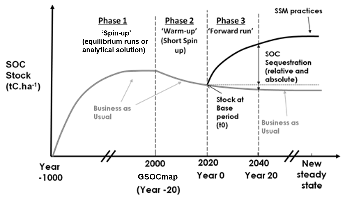
Figure 5.1. SOC stocks simulated in the different phases according to the proposed general modeling procedure.
Table 5.1 Summary of the different modeling phases and data requirements.
| Variables | Phase 1 Long spin up Equilibrium | Phase 2 Short spin up | Phase 3 Forward modeling |
|---|---|---|---|
| Time span | Minimum 500 years (using equilibrium runs procedure) | 20 years | 20 years |
| Infinite (Analytical solution procedure) | |||
| Climatic inputs | 1980-2000 series monthly average: | 2001-2020 year to year monthly data: | 2001-2020 series monthly average: |
| Rain, Temperature, Evaporation/ | Rain, Temperature, Evaporation/ | Rain, Temperature ,Evaporation/ | |
| Evapotranspiration | Evapotranspiration | Evapotranspiration | |
| Soil inputs | Topsoil clay content | Topsoil clay content | Topsoil clay content |
| Initial SOC stocks and pools | Inert organic matter (IOM) as determined by equation 5.2 | Inert organic matter (IOM as determined by equation 5.2 | Inert organic matter (IOM) as determined by equation 5.2 |
| “= 0” for all other fractions (when using equilibrium runs) | Other fractions equal to the final SOC pools modeled in phase 1 | Other fractions equal to the final SOC pools modeled in phase 2 | |
| Carbon inputs | First run : 1tC.ha-1 | NPP | NPP year-to year |
| Adjusted C inputs from equation 5.1 (using equilibrium runs) | year-to year adjusted C inputs, from equation 7 | adjusted C inputs for the BAU, from equation 7 | |
| From equation 5.12 (using analytical solution) | |||
| Estimated from % increase vs. | |||
| BAU for SSM scenarios | |||
| Vegetation cover | Monthly cover determined: by expert opinion, NDVI 2000-2020 or preferred spectral index (see section 3.3.4) | Monthly cover determined: by expert opinion, NDVI 2000-2020 or preferred spectral index (see section 3.3.4) | Monthly cover determined: by expert opinion, NDVI 2000-2020 or preferred spectral index (see section 3.3.4) |
| Land Use | Representative land use of the 1980-2000 period (or layer for year 2000; or best available layer) | Year to year Land use 2000-2020 (or representative land use of the period; or best available layer) | Last available land use layer (e.g. 2015, 2018; 2020) (or best available layer) |
| Modeled Scenarios | BAU | BAU | BAU |
| SSM Low | |||
| SSM Medium | |||
| SSM High | |||
| Expected Results | C inputs at equilibrium | Total SOC and SOC pools at year t=0 (2020) | Total SOC and SOC pools at year t=+20 (2040) for the BAU, and SSMs scenarios |
| Total SOC and SOC pools at year t= -20 (2000) | Absolute and relative Total Sequestration (3 SSMs) | ||
| Absolute and relative Sequestration rates (3 SSMs) | |||
The different data sets required to run the RothC model for the different modeling phases are described in Chapter 6.