Chapter 9 | Stage 1: preparation of input data
This stage is aimed at:
- preparing, organizing and harmonizing all the required input data layers to run the model in the different phases;
- creating supplementary input data layers;
- creating target points for land use classes of interests.
During this stage we will need to arrange and prepare climate datasets for the different modelling phases, generate NPP estimates for each phase, generate vegetation cover data, prepare clay content data layers, and harmonize and stack all layers for each modelling phase. Finally, we will have to create target points to run the model. This stage requires the most effort and is the most time consuming of the entire process. Eleven R scripts, one QGIS script and one Google earth engine script are provided to complete these tasks.
9.1 Preparation of SOC layer
As a default option, users are invited to use the GSOCmap to retrieve their SOC data for their area of interest (AOI). This can be achieved easily, by clipping the GSOCmap to the extent of a shapefile making up the borders of the chosen study area or country. All data sources can be found in Table 6.3 of Chapter 6.
9.1.1 Script Number 0.“SOC_MAP_AOI.R”
Table 9.1 Script Number 0. Preparation of the Soil Organic Carbon SOC layer. Inputs and Outputs
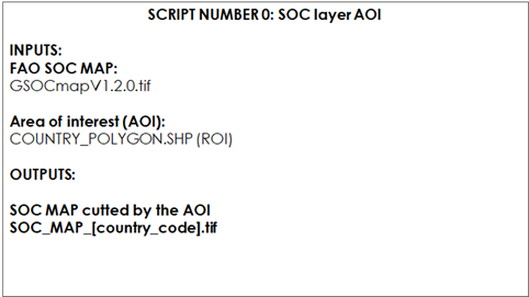
First, open the scrip SOC_MAP_AOI.R in RStudio. If you haven’t done so previously install the necessary packages. Then create two user-defined variables containing the paths to the two working directories: * “WD_AOI” which contains the vector polygon of the AOI; * “WD_GSOC”, which contains the GSOCmap raster layer
#Install all necessary packages
install.packages(c("raster","rgdal","SoilR","Formula","soilassessment","abind","ncdf4"))

#Load the packages into R
library(raster)
library(rgdal)

# Set the path to GSOCmap and Area of interest (AOI) vector.
WD_AOI<-("C:/Training_Material/INPUTS/AOI_POLYGON")
WD_GSOC<-("C:/Training_Material/INPUTS/SOC_MAP")

# Open the shapefile of the AOI (region/country)
setwd(WD_AOI)
AOI<-readOGR("Departamento_Pergamino.shp")

#Open FAO GSOC MAP
setwd(WD_GSOC)
SOC_MAP<-raster("GSOCmap_1.6.1.tif")
Finally, we clip the SOC layer with the vector polygon of the AOI and save the result to the WD_SOC folder. This layer will become the master layer of the process.
SOC_MAP_AOI<-crop(SOC_MAP,AOI)
SOC_MAP_AOI<-mask(SOC_MAP_AOI,AOI)
writeRaster(SOC_MAP_AOI,filename="SOC_MAP_AOI.tif",format="GTiff")
9.2 Preparation of climate Layers
The climate variables needed for the three modeling phases are:
- Monthly rainfall (mm/month);
- Monthly Evapotranspiration (mm/month);
- Average monthly mean air temperature (average \(^\circ\)C/month).
We will need to arrange these climatic variables into three datasets:
- 1980-2000 (monthly average values for the complete series)
- 2001-2020 (year to year monthly values)
- 2001-2020 (monthly average values for the complete series)
Gridded climate data shall be obtained from either National Sources or regional or global datasets when national gridded historical climate datasets are not available. The recommended global data source of these layers are:
- The Climate Research Unit (http://www.cru.uea.ac.uk/)
- TerraClimate (readily available from the Google Earth Engine catalogue: https://developers.google.com/earth-engine/datasets/catalog/IDAHO_EPSCOR_TERRACLIMATE#citations)
For countries wanting to use the TerraClimate or the CRU data set, several scripts to obtain and to reformat the climate spatial layers to run the three modelling phases, will be presented. Users can prepare the necessary input climate data sets using other data sources. However, these scripts may still be helpful to guide the preparation process of other data sets, and as a guide of the required outputs that will be needed as inputs for the different modeling phases. Due to the coarse resolution of the CRU data set, small and/or coastal countries may encounter issues with the data set.
It is important to note that the CRU layers do not cover countries in their entirety. To overcome this, this revised version of the Technical Manual provides two options:
- Perform the whole procedure with higher resolution climate layers again for every point. We have provided scripts to download and prepare TerraClimate climatic layers.
- Re-running the model only for those points that fall outside of the CRU layer using the provided scripts that include a line of code that fills NA values with the average of all surrounding pixel values (Annex).
For both cases a detailed step by step guideline is provided.
The preparation of the climate data depending on whether a user selects the CRU (Option A) or TerraClimate (option B) data set is presented in the flowchart below (Figure 9.0). To make use of the TerraClimate dataset, users need to first download the data for the time periods 1980-2000 and 2001-2018 using two scripts for Google Earth Egine (GEE) and subsequently prepare the target climatic variables using two R scripts.
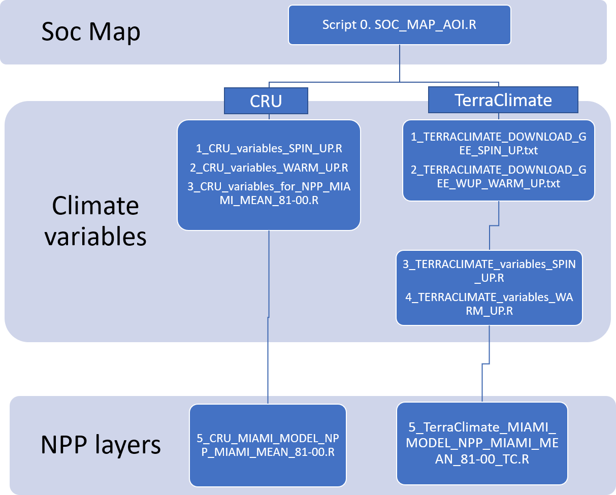
Figure 9.0 Script order to follow depending on wether CRU or TerraClimate data sets are selected
Additionally, in the ANNEX a small guide is provided to overcome issues linked to the use of CRU layers in coastal and small countries.
9.2.1 Option A Preparation of the CRU climatic variables
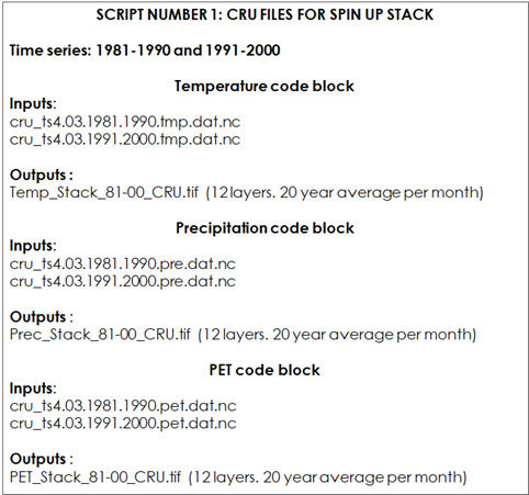
9.2.1.1 Script Number 1. “CRU_variables_SPIN_UP.R”
For each modelling phase we will need a different selection of climate layers. For phase 1 (“Long Spin up”), we will need to stack 12 spatial layers (the output file will be a multiband raster layer) for each climate variable mentioned above (temperature, precipitation and evapotranspiration). The time series for this initial phase goes from 1981 to 2000. The script number 1 will transform the downloaded CRU files to geotiff raster files and obtain monthly averages (temperature, precipitation, evapotranspiration) for the 1981-2000 series, ready to be used in the spin up modelling phase.
Table 9.2 Script Number 1.1 Preparation of CRU datasets for the “Long Spin Up phase”. Inputs and Outputs
Open the script CRU_variables_SPIN_UP.R in RStudio.
The first lines begin with “#”, which indicates that these lines are commented. From line 7 to line 10, the script loads the required packages into R.
library(raster)
library(rgdal)
library(ncdf4)
library(abind)
From line 15 to line 48 the script opens two nc files (1981-1990 and 1991-2000 periods), from a local directory to be defined with the setwd function and converts them into an internal variable called “tmp”. Here we will have to set the path to the local directory of the two temperature files downloaded from the CRU site. Remember to unzip the CRU files.
#Set working directory
#Set working directory
WD<-("C:/Training_Material/INPUTS/CRU_LAYERS")
setwd(WD)

# TEMPERATURE
# Open nc temperature file 1981-1990 unzip the cru files
nc_temp_81_90<-nc_open("cru_ts4.03.1981.1990.tmp.dat.nc")
lon <- ncvar_get(nc_temp_81_90, "lon")
lat <- ncvar_get(nc_temp_81_90, "lat", verbose = F)
t_81_90 <- ncvar_get(nc_temp_81_90, "time")
tmp_81_90<-ncvar_get(nc_temp_81_90, "tmp")
#close de nc temperature file
nc_close(nc_temp_81_90)
# Open nc temperature file 1991-2000
nc_temp_91_00<-nc_open("cru_ts4.03.1991.2000.tmp.dat.nc")
lon <- ncvar_get(nc_temp_91_00, "lon")
lat <- ncvar_get(nc_temp_91_00, "lat", verbose = F)
t_91_00 <- ncvar_get(nc_temp_91_00, "time")
tmp_91_00<-ncvar_get(nc_temp_91_00, "tmp")
#close de nc temperature file
nc_close(nc_temp_91_00)
# Merge 1981-1990 and 1991-2000 data
tmp<-abind(tmp_81_90,tmp_91_00)
Then the script generates a variable to be used later on called “tmp_Jan_1”:
# Get one month temperature ( January)
 tmp_Jan_1<-tmp[,,1]
 dim(tmp_Jan_1)
Now, all the settings for this part of the script are done. The user just has to go on running the rest of the script until the “Precipitation” code begins where “Precipitation” files will be needed. The code below will generate one temperature file, consisting of a stack of 12 raster files with an average of 20 years for each month. Each raster corresponds to a month.
# Create empty list
r<-raster(ncol=3,nrow=3)
Rlist<-list(r,r,r,r,r,r,r,r,r,r,r,r)
 # Average of 20 years (j)  and 12 months (i)
######for loop starts#######
 for (i in 1:12) {
var_sum<-tmp_Jan_1*0
k<-i
 for (j in 1:20) {
print(k)
var_sum<-(var_sum + tmp[,,k])
 k<-k+12
 }
#Save each month average.
 var_avg<-var_sum/20
name<-paste0('Temp_1981_2000_years_avg_',i,'.tif')
 # Make a raster r from each average
ra<- raster(t(var_avg), xmn=min(lon), xmx=max(lon), ymn=min(lat), ymx=max(lat), crs=CRS("+proj=longlat +ellps=WGS84 +datum=WGS84 +no_defs+ towgs84=0,0,0"))
ra<-flip(ra, direction='y')
writeRaster(ra,filename=name, format="GTiff")
Rlist[[i]]<-ra
}
######for loop ends#######
 #save a stack of months averages
 Temp_Stack<-stack(Rlist)
writeRaster(Temp_Stack,filename='Temp_Stack_81-00_CRU.tif',"GTiff")
The first line of the “Precipitation” code block will delete all the variables that have been created until that moment. This will free up memory and increase the execution speed of the rest of the script running.
 #######################################################################################
#PRECIPITATION
 rm(list = ls())
WD<-("C:/Training_Material/INPUTS/CRU_LAYERS")
setwd(WD)
From line 106 to line 144, the script operates in the same way as for the initial “Temperature” code block. We must define the path to the CRU precipitation files and run the rest of the code:
 # Open nc precipitation file 1981-1990
nc_pre_81_90<-nc_open("cru_ts4.03.1981.1990.pre.dat.nc")
 lon <- ncvar_get(nc_pre_81_90, "lon")
lat <- ncvar_get(nc_pre_81_90, "lat", verbose = F)
t <- ncvar_get(nc_pre_81_90, "time")
 pre_81_90<-ncvar_get(nc_pre_81_90, "pre")
 #close de nc temperature file
 nc_close(nc_pre_81_90)
# Open nc precipitation file 1991-2000
nc_pre_91_00<-nc_open("cru_ts4.03.1991.2000.pre.dat.nc")
 lon <- ncvar_get(nc_pre_91_00, "lon")
lat <- ncvar_get(nc_pre_91_00, "lat", verbose = F)
t <- ncvar_get(nc_pre_91_00, "time")
 pre_91_00<-ncvar_get(nc_pre_91_00, "pre")
 #close de nc temperature file
 nc_close(nc_pre_91_00)
 # Merge 1981-1990 and 1991-2000 data
 pre_81_00<-abind(pre_81_90,pre_91_00)
# Have one month Precipitation ( January)
 pre_Jan_1<-pre_81_00[,,1]
 dim(pre_Jan_1)
The following code block is very similar to the one used to create the temperature files, but instead of creating an annual average, the script saves the average of the monthly sum.
 # Create empty list
r<-raster(ncol=3,nrow=3)
Rlist<-list(r,r,r,r,r,r,r,r,r,r,r,r)
 # Average of 20 years (j)  and 12 months (i)
######for loop starts#######
 for (i in 1:12) {
var_sum<-pre_Jan_1*0
k<-i
 for (j in 1:20) {
print(k)
var_sum<-(var_sum + pre_81_00[,,k])
 k<-k+12
 }
#Save each month average.
 var_avg<-var_sum/20
name<-paste0('Prec_1981_2000_years_avg_',i,'.tif')
 # Make a raster r from the each average
ra<- raster(t(var_avg), xmn=min(lon), xmx=max(lon), ymn=min(lat), ymx=max(lat), crs=CRS("+proj=longlat +ellps=WGS84 +datum=WGS84 +no_defs+ towgs84=0,0,0"))
ra<-flip(ra, direction='y')
writeRaster(ra,filename=name, format="GTiff")
Rlist[[i]]<-ra
}
######for loop ends#######
 #save a stack of months averages
Prec_Stack<-stack(Rlist)
writeRaster(Prec_Stack,filename='Prec_Stack_81-00_CRU.tif',"GTiff")
Finally, we must run the “Potential Evapotranspiration” block of the script. First, as we did before, we should delete the variables created in the “Precipitation” code block.
########################################################################
# POTENTIAL EVAPOTRANSPIRATION
 rm(list = ls())
WD<-("C:/Training_Material/INPUTS/CRU_LAYERS")
setwd(WD)
The same commands are repeated as the ones executed for the previous code blocks: "Temperature" and "Precipitation".
# Open nc temperature file 81 - 90
nc_pet_81_90<-nc_open("cru_ts4.03.1981.1990.pet.dat.nc")
 lon <- ncvar_get(nc_pet_81_90, "lon")
lat <- ncvar_get(nc_pet_81_90, "lat", verbose = F)
t <- ncvar_get(nc_pet_81_90, "time")
 pet_81_90<-ncvar_get(nc_pet_81_90, "pet")
 #close de nc temperature file
 nc_close(nc_pet_81_90)
 # Open nc temperature file 91 - 00
 nc_pet_91_00<-nc_open("cru_ts4.03.1991.2000.pet.dat.nc")
 lon <- ncvar_get(nc_pet_91_00, "lon")
lat <- ncvar_get(nc_pet_91_00, "lat", verbose = F)
t <- ncvar_get(nc_pet_91_00, "time")
 pet_91_00<-ncvar_get(nc_pet_91_00, "pet")
 #close de nc temperature file
 nc_close(nc_pet_91_00)
 # Merge 1981-1990 and 1991-2000 data
 pet_81_00<-abind(pet_81_90,pet_91_00)
# Have one month ETP ( January)
 pet_Jan_1<-pet_81_90[,,1]
 dim(pet_Jan_1)
 # Create empty list
r<-raster(ncol=3,nrow=3)
Rlist<-list(r,r,r,r,r,r,r,r,r,r,r,r)
 # Average of 8 years (j)  and 12 months (i)
######for loop starts#######
 for (i in 1:12) {
var_sum<-pet_Jan_1*0
k<-i

for (j in 1:20) {
print(k)
var_sum<-(var_sum + pet_81_00[,,k])
 k<-k+12
 }
#Save each month average.
 var_avg<-var_sum*30/20
name<-paste0('PET_1981_2000_years_avg_',i,'.tif')
 # Make a raster r from the each average
ra<- raster(t(var_avg), xmn=min(lon), xmx=max(lon), ymn=min(lat), ymx=max(lat), crs=CRS("+proj=longlat +ellps=WGS84 +datum=WGS84 +no_defs+ towgs84=0,0,0"))
ra<-flip(ra, direction='y')
writeRaster(ra,filename=name, format="GTiff")
Rlist[[i]]<-ra
}
######for loop ends#######
 #save a stack of months averages
 PET_Stack<-stack(Rlist)
writeRaster(PET_Stack,filename='PET_Stack_81-00_CRU.tif',"GTiff")
Script number 1 is completed. The user should have created two files for the Temperature variable, two for the Precipitation variable and one for ETP variable. All these files will be used to create a raster stack of all layers needed to run the “long spin up” phase.
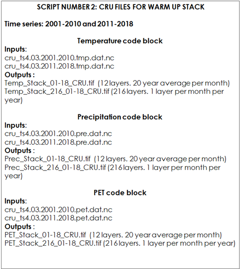
9.2.1.2 Script Number 2. “CRU_variables_WARM_UP.R”
The purpose of the “Warm up” phase is to adjust the initial SOC stock and initial pools for the “forward” phase. Once the input climate layers have been harmonized, the model will run for each year from 2001 to 2018/20, using the monthly climate data of each year of the series (for 216/240 values for each month of the time series). The script number 2 is prepared to arrange the necessary CRU climate files for this phase. We will need to generate one raster stack of 216/240 spatial layers for each climate variable mentioned above (216 spatial layers if we use just 18 years period instead of a 20 year period; from 2001 to 2018, depending on the available climate data). Each stack will have one layer for each month from 2001 to 2018/2020. For phase number 3, the “Forward” phase, we will need monthly averages of the time series 2001-2018/20. We will use the same arrangement as used in phase number one (one stack of 12 bands for each variable) but instead of using the averages of the 1981-2000 period we will use the climatic data of the 2001-2018/20 period. We will assume that there is no climate change in the next 20 years. Thus, script number 2 will also prepare the climate files for the “forward phase”.
Table 9.3 Overview of the input and output files in script number 1.2 used for the files for Warm Up and Forward Phases.
First, we must load the required R packages.
library(raster)
library(rgdal)
library(ncdf4)
library(abind)
Then we will have to define the path directory to the CRU files.
# TEMPERATURE
WD<-("C:/Training_Material/INPUTS/CRU_LAYERS")
setwd(WD)
 # Open nc temperature file 2001-2010
nc_temp_01_10<-nc_open("cru_ts4.03.2001.2010.tmp.dat.nc")
 lon <- ncvar_get(nc_temp_01_10, "lon")
lat <- ncvar_get(nc_temp_01_10, "lat", verbose = F)
t_01_10 <- ncvar_get(nc_temp_01_10, "time")
 tmp_01_10<-ncvar_get(nc_temp_01_10, "tmp")
 #close de nc temperature file
 nc_close(nc_temp_01_10)
 # Open nc temperature file 2010-2018
nc_temp_11_18<-nc_open("cru_ts4.03.2011.2018.tmp.dat.nc")
 lon <- ncvar_get(nc_temp_11_18, "lon")
lat <- ncvar_get(nc_temp_11_18, "lat", verbose = F)
t_11_18 <- ncvar_get(nc_temp_11_18, "time")
 tmp_11_18<-ncvar_get(nc_temp_11_18, "tmp")
 #close de nc temperature file
 nc_close(nc_temp_11_18)
 # Merge 2001-2010 and 2011-2018 data
 tmp<-abind(tmp_01_10,tmp_11_18)
 # Have one month temperature ( January)
 tmp_Jan_1<-tmp[,,1]
 dim(tmp_Jan_1)
The next code block will create two raster stacks: a temperature monthly average for the 18/20 year period, and a file with one layer per month per year, summarizing 216 layers in the stack.
# Create empty list
r<-raster(ncol=3,nrow=3)
Rlist<-list(r,r,r,r,r,r,r,r,r,r,r,r)
 # Average of 20 years (j)  and 12 months (i)
##########for loop starts###############
 for (i in 1:12) {
var_sum<-tmp_Jan_1*0
k<-i
for (j in 1:(dim(tmp)[3]/12)) {
print(k)
var_sum<-(var_sum + tmp[,,k])
 k<-k+12
 }
#Save each month average.
 var_avg<-var_sum/(dim(tmp)[3]/12)
name<-paste0('Temp_2001_2018_years_avg_',i,'.tif')
 # Make a raster r from each average
ra<- raster(t(var_avg), xmn=min(lon), xmx=max(lon), ymn=min(lat), ymx=max(lat), crs=CRS("+proj=longlat +ellps=WGS84 +datum=WGS84 +no_defs+ towgs84=0,0,0"))
ra<-flip(ra, direction='y')
#writeRaster(ra,filename=name, format="GTiff")
Rlist[[i]]<-ra
}
##########for loop ends###############
 #save a stack of months averages
 Temp_Stack<-stack(Rlist)
writeRaster(Temp_Stack,filename='Temp_Stack_01-18_CRU.tif',"GTiff")
 # SAVE 1 layer per month per year
 Rlist2-Rlist
##########for loop starts###############
 for (q in 1:(dim(tmp)[3])) {
print(q)
var<-(tmp[,,q])
 #Save each month average.
 name<-paste0('Temp_2001-2018',q,'.tif')
 # Make a raster r from each average
ra<- raster(t(var), xmn=min(lon), xmx=max(lon), ymn=min(lat), ymx=max(lat), crs=CRS("+proj=longlat +ellps=WGS84 +datum=WGS84 +no_defs+ towgs84=0,0,0"))
ra<-flip(ra, direction='y')
#writeRaster(ra,filename=name, format="GTiff")
Rlist2[[q]]<-ra
}
##########for loop ends###############

Temp_Stack_2<-stack(Rlist2)
writeRaster(Temp_Stack_2,filename='Temp_Stack_216_01-18_CRU.tif',"GTiff")
 #PRECIPITATION
 rm(list = ls())
WD<-("C:/Training_Material/INPUTS/CRU_LAYERS")
setwd(WD)
 # Open nc precipitation file 2001-2010
nc_pre_01_10<-nc_open("cru_ts4.03.2001.2010.pre.dat.nc")
 lon <- ncvar_get(nc_pre_01_10, "lon")
lat <- ncvar_get(nc_pre_01_10, "lat", verbose = F)
t <- ncvar_get(nc_pre_01_10, "time")
 pre_01_10<-ncvar_get(nc_pre_01_10, "pre")
 #close de nc temperature file
 nc_close(nc_pre_01_10)
 # Open nc precipitation file 2011-2018
nc_pre_11_18<-nc_open("cru_ts4.03.2011.2018.pre.dat.nc")
 lon <- ncvar_get(nc_pre_11_18, "lon")
lat <- ncvar_get(nc_pre_11_18, "lat", verbose = F)
t <- ncvar_get(nc_pre_11_18, "time")
 pre_11_18<-ncvar_get(nc_pre_11_18, "pre")
 #close de nc temperature file
 nc_close(nc_pre_11_18)
 # Merge 2001-2010 and 2011-2018 data
 pre_01_18<-abind(pre_01_10,pre_11_18)
# Have one month Precipitation ( January)
 pre_Jan_1<-pre_01_18[,,1]
 dim(pre_Jan_1)
 Continue running until the end of the block:
 # Create empty list
r<-raster(ncol=3,nrow=3)
Rlist<-list(r,r,r,r,r,r,r,r,r,r,r,r)
Rlist2<-Rlist
 # Average of 20 years (j)  and 12 months (i)
#########for loop starts############
 for (i in 1:12) {
var_sum<-pre_Jan_1*0
k<-i
 for (j in 1:(dim(pre_01_18)[3]/12)) {
print(k)
var_sum<-(var_sum + pre_01_18[,,k])
 k<-k+12
 }
#Save each month average.
 var_avg<-var_sum/(dim(pre_01_18)[3]/12)
 name<-paste0('Prec_2001_2018_years_avg_',i,'.tif')
 # Make a raster r from  each average
ra<- raster(t(var_avg), xmn=min(lon), xmx=max(lon), ymn=min(lat), ymx=max(lat), crs=CRS("+proj=longlat +ellps=WGS84 +datum=WGS84 +no_defs+ towgs84=0,0,0"))
ra<-flip(ra, direction='y')
#writeRaster(ra,filename=name, format="GTiff")
Rlist[[i]]<-ra
}
#########for loop ends############
 #save a stack of months averages
 Prec_Stack<-stack(Rlist)
writeRaster(Prec_Stack,filename='Prec_Stack_01-18_CRU.tif',"GTiff")
 # SAVE 1 layer per month per year
#########for loop starts############
 for (q in 1:(dim(pre_01_18)[3])) {
print(q)
var<-(pre_01_18[,,q])
 #Save each month average.
 name<-paste0('Prec_2001-2018',q,'.tif')
 # Make a raster r from each average
ra<- raster(t(var), xmn=min(lon), xmx=max(lon), ymn=min(lat), ymx=max(lat), crs=CRS("+proj=longlat +ellps=WGS84 +datum=WGS84 +no_defs+ towgs84=0,0,0"))
ra<-flip(ra, direction='y')
#writeRaster(ra,filename=name, format="GTiff")
Rlist2[[q]]<-ra
}
#########for loop ends############
Prec_Stack_2<-stack(Rlist2)
writeRaster(Prec_Stack_2,filename='Prec_Stack_216_01-18_CRU.tif',"GTiff")
Now we must run the PET block. We will then run the rest of the code to create the necessary tif files.
########################################################################
# POTENTIAL EVAPOTRANSPIRATION
rm(list = ls())
WD<-("C:/Training_Material/INPUTS/CRU_LAYERS")
setwd(WD)
# Open nc temperature file 01 - 10
nc_pet_01_10<-nc_open("cru_ts4.03.2001.2010.pet.dat.nc")
lon <- ncvar_get(nc_pet_01_10, "lon")
lat <- ncvar_get(nc_pet_01_10, "lat", verbose = F)
t <- ncvar_get(nc_pet_01_10, "time")
pet_01_10<-ncvar_get(nc_pet_01_10, "pet")
#close de nc temperature file
nc_close(nc_pet_01_10)
# Open nc temperature file 11 - 18 nc_pet_11_18<-nc_open("cru_ts4.03.2011.2018.pet.dat.nc")
lon <- ncvar_get(nc_pet_11_18, "lon")
lat <- ncvar_get(nc_pet_11_18, "lat", verbose = F)
t <- ncvar_get(nc_pet_11_18, "time")
pet_11_18<-ncvar_get(nc_pet_11_18, "pet")
#close de nc temperature file
nc_close(nc_pet_11_18)
# Merge 2001-2010 and 2011-2018 data
pet_01_18<-abind(pet_01_10,pet_11_18)
# get one month ETP ( January)
pet_Jan_1<-pet_01_18[,,1]
dim(pet_Jan_1)
# Create empty list
r<-raster(ncol=3,nrow=3)
Rlist<-list(r,r,r,r,r,r,r,r,r,r,r,r)
Rlist2<-Rlist
# Average of 18 years (j) and 12 months (i)
############for loop starts##############
for (i in 1:12) {
var_sum<-pet_Jan_1*0
k<-i
for (j in 1:(dim(pet_01_18)[3]/12)) {
print(k)
var_sum<-(var_sum + pet_01_18[,,k])
k<-k+12
}
#Save each month average.
var_avg<-var_sum*30/(dim(pet_01_18)[3]/12)
name<-paste0('PET_2001_2018_years_avg_',i,'.tif')
# Make a raster r from the each average
ra<- raster(t(var_avg), xmn=min(lon), xmx=max(lon), ymn=min(lat), ymx=max(lat), crs=CRS("+proj=longlat +ellps=WGS84 +datum=WGS84 +no_defs+ towgs84=0,0,0"))
ra<-flip(ra, direction='y')
#writeRaster(ra,filename=name, format="GTiff")
Rlist[[i]]<-ra
}
############for loop ends##############
#save a stack of months averages
PET_Stack<-stack(Rlist)
writeRaster(PET_Stack,filename='PET_Stack_01-18_CRU.tif',"GTiff")
# SAVE 1 layer per month per year
############for loop starts##############
for (q in 1:(dim(pet_01_18)[3])) {
print(q)
var<-(pet_01_18[,,q])*30
#Save each month average.
name<-paste0('PET_2001-2018',q,'.tif')
# Make a raster r from each average
ra<- raster(t(var), xmn=min(lon), xmx=max(lon), ymn=min(lat), ymx=max(lat), crs=CRS("+proj=longlat +ellps=WGS84 +datum=WGS84 +no_defs+ towgs84=0,0,0"))
ra<-flip(ra, direction='y')
writeRaster(ra,filename=name, format="GTiff")
Rlist2[[q]]<-ra
}
############for loop starts##############
PET_Stack_2<-stack(Rlist2)
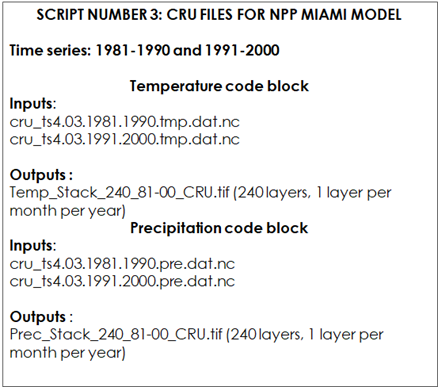
writeRaster(PET_Stack_2,filename='PET_Stack_216_01-18_CRU.tif',"GTiff") 9.2.1.3 Script Number 3. Preparation of CRU files to estimate NPP 1981-2000
We will need to convert the CRU monthly climate data 1981-2000 into annual data to estimate annual NPP 1981-2000.The script number 3 will process the CRU files from the 1981-2000 series to generate the climate inputs files required to estimate NPP by the MIAMI model.
Table 9.4. Script Number 1.3. CRU files for MIAMI MODEL. Inputs and Outputs
We will first open the R file: “CRU_variables_for_NPP_MIAMI_MEAN_81-00.R” and load the required packages:
library(raster)
library(rgdal)
library(ncdf4)
library(abind)
The first block is the “temperature” block. We must set the path to the CRU files.
# TEMPERATURE
WD<-("C:/Training_Material/INPUTS/CRU_LAYERS")
setwd(WD)
 # Open nc temperature file 1981-1990
nc_temp_81_90<-nc_open("cru_ts4.03.1981.1990.tmp.dat.nc")
 lon <- ncvar_get(nc_temp_81_90, "lon")
lat <- ncvar_get(nc_temp_81_90, "lat", verbose = F)
t_81_90 <- ncvar_get(nc_temp_81_90, "time")
 tmp_81_90<-ncvar_get(nc_temp_81_90, "tmp")
 #close de nc temperature file
 nc_close(nc_temp_81_90)
 # Open nc temperature file 1991-2000
nc_temp_91_00<-nc_open("cru_ts4.03.1991.2000.tmp.dat.nc")
 lon <- ncvar_get(nc_temp_91_00, "lon")
lat <- ncvar_get(nc_temp_91_00, "lat", verbose = F)
t_91_00 <- ncvar_get(nc_temp_91_00, "time")
 tmp_91_00<-ncvar_get(nc_temp_91_00, "tmp")
 #close de nc temperature file
 nc_close(nc_temp_91_00)
 # Merge 1981-1990 and 1991-2000 data
 tmp<-abind(tmp_81_90,tmp_91_00)
 # Get one month temperature ( January)

tmp_Jan_1<-tmp[,,1]
 dim(tmp_Jan_1)
# Create empty list
r<-raster(ncol=3,nrow=3)
Rlist<-list(r,r,r,r,r,r,r,r,r,r,r,r)
 # SAVE 1 layer per month per year
 Rlist2<-Rlist
############for loop starts###########
 for (q in 1:(dim(tmp)[3])) {
var<-(tmp[,,q])
 #Save each month average.
 name<-paste0('Temp_1981-2000',q,'.tif')
 # Make a raster r from each average
ra<- raster(t(var), xmn=min(lon), xmx=max(lon), ymn=min(lat), ymx=max(lat), crs=CRS("+proj=longlat +ellps=WGS84 +datum=WGS84 +no_defs+ towgs84=0,0,0"))
ra<-flip(ra, direction='y')
#writeRaster(ra,filename=name, format="GTiff")
Rlist2[[q]]<-ra
}
############for loop ends###########
Temp_Stack_2<-stack(Rlist2)
writeRaster(Temp_Stack_2,filename='Temp_Stack_240_81-00_CRU.tif',"GTiff")
After that, the “precipitation” block begins.
#PRECIPITATION
rm(list = ls())
WD<-("C:/Training_Material/INPUTS/CRU_LAYERS")
setwd(WD)
# Open nc precipitation file 1981-1990
nc_pre_81_90<-nc_open("cru_ts4.03.1981.1990.pre.dat.nc")
lon <- ncvar_get(nc_pre_81_90, "lon")
lat <- ncvar_get(nc_pre_81_90, "lat", verbose = F)
t <- ncvar_get(nc_pre_81_90, "time")
pre_81_90<-ncvar_get(nc_pre_81_90, "pre")
#close de nc temperature file
nc_close(nc_pre_81_90)
# Open nc precipitation file 1991-2000
nc_pre_91_00<-nc_open("cru_ts4.03.1991.2000.pre.dat.nc")
lon <- ncvar_get(nc_pre_91_00, "lon")
lat <- ncvar_get(nc_pre_91_00, "lat", verbose = F)
t <- ncvar_get(nc_pre_91_00, "time")
pre_91_00<-ncvar_get(nc_pre_91_00, "pre")
#close de nc temperature file
nc_close(nc_pre_91_00)
# Merge 1981-1990 and 1991-2000 data
pre_81_00<-abind(pre_81_90,pre_91_00)
# Create empty list
r<-raster(ncol=3,nrow=3)
Rlist<-list(r,r,r,r,r,r,r,r,r,r,r,r)
Rlist2<-Rlist
# SAVE 1 layer per month per year
##############for loop starts############
for (q in 1:(dim(pre_81_00)[3])) {
var<-(pre_81_00[,,q])
#Save each month average.
#name<-paste0('Prec_2001-2018',q,'.tif')
# Make a raster r from each average
ra<- raster(t(var), xmn=min(lon), xmx=max(lon), ymn=min(lat), ymx=max(lat), crs=CRS("+proj=longlat +ellps=WGS84 +datum=WGS84 +no_defs+ towgs84=0,0,0"))
ra<-flip(ra, direction='y')
#writeRaster(ra,filename=name, format="GTiff")
Rlist2[[q]]<-ra
}
##############for loop ends############
Prec_Stack_2<-stack(Rlist2)
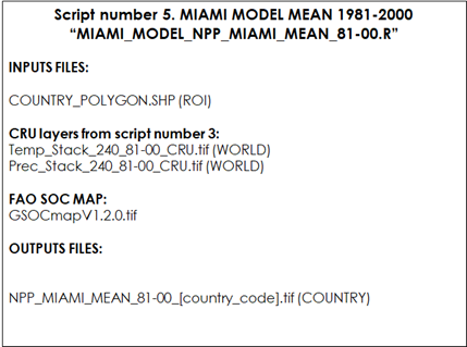
writeRaster(Prec_Stack_2,filename='Prec_Stack_240_81-00_CRU.tif',"GTiff")9.2.1.4 Script Number 5. CRU MIAMI model NPP mean (1981-2000)
To adjust yearly C inputs during the warm up phase according to annual NPP values, we will need to estimate an average annual NPP 1981-2000, that will be used as the starting point to adjust C inputs during the “warm up” phase (See chapter 6). Script number 5 uses the climate raster outputs from script number 3 and estimates an annual NPP mean 1981-2000 value.
Table 9.5 Script Number 5. CRU Miami Model 81-00 Mean. Inputs and Outputs
First, we will need to open the R script: “MIAMI_MODEL_NPP_MIAMI_MEAN_81-00.R” Analogously to the previous scripts, the first lines load the required packages into R and set the working directories. Then the annual precipitation and annual temperature stacks (1981-2000) that were created in script number 3 are opened:
library(raster)
library(rgdal)
WD_NPP<-("C:/Training_Material/INPUTS/NPP")

WD_AOI<-("C:/Training_Material/INPUTS/AOI_POLYGON")
WD_GSOC<-("C:/Training_Material/INPUTS/SOC_MAP")
WD_CRU_LAYERS<-("C:/Training_Material/INPUTS/CRU_LAYERS")
setwd(WD_CRU_LAYERS)
# Open Annual Precipitation (mm) and Mean Annual Temperature (degree C) stacks
Temp<-stack("Temp_Stack_240_81-00_CRU.tif")
Prec<- stack("Prec_Stack_240_81-00_CRU.tif")
At line 73 the user must set the output directory to save the output files.
# Temperature Annual Mean
k<-1
TempList<-list()
#######loop for starts#########
for (i in 1:20){
Temp1<-mean(Temp[[k:(k+11)]])
TempList[i]<-Temp1
k<-k+12
}
#######loop for ends##########
TempStack<-stack(TempList)
#Annual Precipitation

k<-1
PrecList<-list()
########loop for starts#######
for (i in 1:20){
Prec1<-sum(Prec[[k:(k+11)]])
PrecList[i]<-Prec1
k<-k+12
}
########loop for ends#######
PrecStack<-stack(PrecList)
# Calculate eq 1 from MIAMI MODEL (g DM/m2/day)
NPP_Prec<-3000*(1-exp(-0.000664*PrecStack))
# Calculate eq 2 from MIAMI MODEL (g DM/m2/day)
NPP_temp<-3000/(1+exp(1.315-0.119*TempStack))
# Calculate eq 3 from MIAMI MODEL (g DM/m2/day)
NPP_MIAMI_List<-list()
########loop for starts#######
for (i in 1:20){
NPP_MIAMI_List[i]<-min(NPP_Prec[[i]],NPP_temp[[i]])
}
########loop for ends#######
NPP_MIAMI<-stack(NPP_MIAMI_List)

#NPP_MIAMI gDM/m2/year To tn DM/ha/year
NPP_MIAMI_tnDM_Ha_Year<-NPP_MIAMI*(1/100)
#NPP_MIAMI tn DM/ha/year To tn C/ha/year
NPP_MIAMI_tnC_Ha_Year<-NPP_MIAMI_tnDM_Ha_Year*0.5
# Save WORLD NPP MIAMI MODEL tnC/ha/year
setwd(WD_NPP)
writeRaster(NPP_MIAMI_tnC_Ha_Year,filename="NPP_MIAMI_tnC_Ha_Year_STACK_81-00.tif",format="GTiff")
# NPP MEAN
NPP_MIAMI_MEAN_81_00<-mean(NPP_MIAMI_tnC_Ha_Year)

Then we will need to open the country polygon vector and the latest version of the FAO GSOCmap.
## Open the shapefile of the region/country
setwd(WD_AOI)
AOI<-readOGR("Departamento_Pergamino.shp")
#Open FAO GSOC MAP
setwd(WD_GSOC)
SOC_MAP_AOI<-raster("SOC_MAP_AOI.tif")
# Crop & mask
setwd(WD_NPP)
NPP_MIAMI_MEAN_81_00_AOI<-crop(NPP_MIAMI_MEAN_81_00,AOI)
NPP_MIAMI_MEAN_81_00_AOI<-resample(NPP_MIAMI_MEAN_81_00_AOI,SOC_MAP_AOI)
NPP_MIAMI_MEAN_81_00_AOI<-mask(NPP_MIAMI_MEAN_81_00_AOI,AOI)

writeRaster(NPP_MIAMI_MEAN_81_00_AOI,filename="NPP_MIAMI_MEAN_81-00_AOI.tif",format="GTiff")
In order to estimate the uncertainty of our predictions, we will create two additional layers, but this time using a minimum and maximum combination of precipitation and temperature variables to generate minimum and maximum NPP layers (See Chapter 12).
#UNCERTAINTIES MINIMUM TEMP , PREC
Temp_min<-Temp*1.02
Prec_min<-Prec*0.95
# Temperature Annual Mean
k<-1
TempList<-list()
########loop for starts#######
for (i in 1:20){
Temp1<-mean(Temp_min[[k:(k+11)]])
TempList[i]<-Temp1
k<-k+12
}
########loop for ends#######
TempStack<-stack(TempList)
#Annual Precipitation
k<-1
PrecList<-list()
########loop for starts#######
for (i in 1:20){
Prec1<-sum(Prec_min[[k:(k+11)]])
PrecList[i]<-Prec1
k<-k+12
}
########loop for ends#######
PrecStack<-stack(PrecList)
# Calculate eq 1 from MIAMI MODEL (g DM/m2/day)
NPP_Prec<-3000*(1-exp(-0.000664*PrecStack))
# Calculate eq 2 from MIAMI MODEL (g DM/m2/day)
NPP_temp<-3000/(1+exp(1.315-0.119*TempStack))
# Calculate eq 3 from MIAMI MODEL (g DM/m2/day)
NPP_MIAMI_List<-list()
########loop for starts#######
for (i in 1:20){
NPP_MIAMI_List[i]<-min(NPP_Prec[[i]],NPP_temp[[i]])
}
########loop for ends#######
NPP_MIAMI<-stack(NPP_MIAMI_List)
#NPP_MIAMI gDM/m2/year To tn DM/ha/year
NPP_MIAMI_tnDM_Ha_Year<-NPP_MIAMI*(1/100)
#NPP_MIAMI tn DM/ha/year To tn C/ha/year

NPP_MIAMI_tnC_Ha_Year<-NPP_MIAMI_tnDM_Ha_Year*0.5
# Save WORLD NPP MIAMI MODEL tnC/ha/year
setwd(WD_NPP)
writeRaster(NPP_MIAMI_tnC_Ha_Year,filename="NPP_MIAMI_tnC_Ha_Year_STACK_81-00_MIN.tif",format="GTiff")
# NPP MEAN
NPP_MIAMI_MEAN_81_00<-mean(NPP_MIAMI_tnC_Ha_Year)
# Crop & and mask
setwd(WD_NPP)
NPP_MIAMI_MEAN_81_00_AOI<-crop(NPP_MIAMI_MEAN_81_00,AOI)
NPP_MIAMI_MEAN_81_00_AOI<-resample(NPP_MIAMI_MEAN_81_00_AOI,SOC_MAP_AOI)
NPP_MIAMI_MEAN_81_00_AOI<-mask(NPP_MIAMI_MEAN_81_00_AOI,AOI)
writeRaster(NPP_MIAMI_MEAN_81_00_AOI,filename="NPP_MIAMI_MEAN_81-00_AOI_MIN.tif",format="GTiff")
#UNCERTAINTIES MAXIMUM TEMP , PREC
# Open Anual Precipitation (mm) and Mean Anual Temperature (grades C) stacks
Temp_max<-Temp*0.98
Prec_max<-Prec*1.05
# Temperature Annual Mean
k<-1
TempList<-list()
########loop for starts#######
for (i in 1:20){

Temp1<-mean(Temp_max[[k:(k+11)]])
TempList[i]<-Temp1
k<-k+12
}
########loop for ends#######
TempStack<-stack(TempList)
#Annual Precipitation
k<-1
PrecList<-list()
########loop for starts#######
for (i in 1:20){
Prec1<-sum(Prec_max[[k:(k+11)]])
PrecList[i]<-Prec1
k<-k+12
}
########loop for ends#######
PrecStack<-stack(PrecList)
# Calculate eq 1 from MIAMI MODEL (g DM/m2/day)
NPP_rain<-3000*(1-exp(-0.000664*PrecStack))
# Calculate eq 2 from MIAMI MODEL (g DM/m2/day)
NPP_temp<-3000/(1+exp(1.315-0.119*TempStack))

# Calculate eq 3 from MIAMI MODEL (g DM/m2/day)
NPP_MIAMI_List<-list()
########loop for starts#######
for (i in 1:20){
NPP_MIAMI_List[i]<-min(NPP_Prec[[i]],NPP_temp[[i]])
}
########loop for ends#######
NPP_MIAMI<-stack(NPP_MIAMI_List)
#NPP_MIAMI gDM/m2/year To tn DM/ha/year
NPP_MIAMI_tnDM_Ha_Year<-NPP_MIAMI*(1/100)
#NPP_MIAMI tn DM/ha/year To tn C/ha/year
NPP_MIAMI_tnC_Ha_Year<-NPP_MIAMI_tnDM_Ha_Year*0.5
# Save NPP MIAMI MODEL tnC/ha/year
setwd(WD_NPP)
writeRaster(NPP_MIAMI_tnC_Ha_Year,filename="NPP_MIAMI_tnC_Ha_Year_STACK_81-00_MAX.tif",format="GTiff")
# NPP MEAN
NPP_MIAMI_MEAN_81_00<-mean(NPP_MIAMI_tnC_Ha_Year)
# Crop & and mask
setwd(WD_NPP)
NPP_MIAMI_MEAN_81_00_AOI<-crop(NPP_MIAMI_MEAN_81_00,AOI)
NPP_MIAMI_MEAN_81_00_AOI<-resample(NPP_MIAMI_MEAN_81_00_AOI,SOC_MAP_AOI)
NPP_MIAMI_MEAN_81_00_AOI<-mask(NPP_MIAMI_MEAN_81_00_AOI,AOI)

writeRaster(NPP_MIAMI_MEAN_81_00_AOI,filename="NPP_MIAMI_MEAN_81-00_AOI_MAX.tif",format="GTiff")
9.2.2 Option B Preparation of the TerraClimate climatic variables
This section presents step by step guidelines on how to download and prepare the required climatic variables from the TerraClimate data set.
9.2.2.1 Script Number 1. TerraClimate GEE Spin up phase
The TerraClimate data set can be downloaded directly from Google Earth Engine, a powerful and free cloud computing platform. First, the user will need to activate a Google Earth Engine account. To run the Google Earth Engine (GEE) tool, the user will need to copy and paste the script (provided below) into the GEE code editor (central panel, Fig. 9.1).
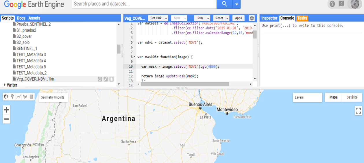
Figure 9.1 Google Earth Engine code editor
To run the script the user can input a new geometry using the geometry tools panel (Figure 9.2) or by uploading a shapefile.
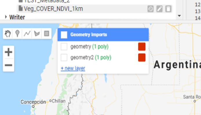
Figure 9.2 Drawing a polygon in Google Earth Engine
The following script can be copied and pasted into GEE without any further modifications:
// Climate data sets for the Spin Up phase 1980-2001
// calculate the average temperature from minimum and maximum temperatures
// download the Minimum and Maximum Temperature
// download the Average temperature
// download the PET
// download the Precipitation

var dataset = ee.ImageCollection('IDAHO_EPSCOR/TERRACLIMATE')
                  .filter(ee.Filter.date('1981-01-01', '2001-01-01'));

var maximumTemperature = dataset.select('tmmx');
var mxT = maximumTemperature.toBands();
var minimumTemperature = dataset.select('tmmn');
var mnT = minimumTemperature.toBands();

var precipitation =dataset.select('pr');
var pre =precipitation.toBands();

var evapotranspiration = dataset.select('pet');
var pet =evapotranspiration.toBands();

var diff = mxT.add(mnT);
var avT = diff.divide(2);

var avT =avT.clip(geometry);
var pre =pre.clip(geometry);
var pet =pet.clip(geometry);


Map.addLayer(avT, {}, 'default RGB');
Map.addLayer(pre, {}, 'default RGB');
Map.addLayer(pet, {}, 'default RGB');


var regionJSON = JSON.stringify(avT.getInfo());
Export.image.toDrive({
          image: avT,
          folder: "TerraClimate",
          description: 'AverageTemperature_1981-2001',
          scale: 4000,
          region: geometry
});

var regionJSON = JSON.stringify(pre.getInfo());
Export.image.toDrive({
          image: pre,
          folder: "TerraClimate",
          description: 'Precipitation_1981-2001',
          scale: 4000,
          region: geometry
});

var regionJSON = JSON.stringify(pet.getInfo());
Export.image.toDrive({
          image: pet,
          folder: "TerraClimate",
          description: 'PET_1981-2001',
          scale: 4000,
          region: geometry
});
9.2.2.2 Scrip Number 2. TerraClimate GEE Warm up and Forward phase
To retrieve the necessary climatic data (2001-2018/20) to be used as input for the warm up and subsequent forward phase the same steps are repeated as for Script 2.1. After defining a geometry or inputting a shapefile the following code can be copied and pasted into the GEE code editor.
/ Climate data sets for the Warm Up phase and Forward phase 2001 - 2020
// calculate the average temperature from minimum and maximum temperatures
// download the Average temperature
// download the PET
// download the Precipitation

var dataset = ee.ImageCollection('IDAHO_EPSCOR/TERRACLIMATE')
                  .filter(ee.Filter.date('2001-01-01', '2020-01-01'));

var maximumTemperature = dataset.select('tmmx');
var mxT = maximumTemperature.toBands();
var minimumTemperature = dataset.select('tmmn');
var mnT = minimumTemperature.toBands();

var precipitation =dataset.select('pr');
var pre =precipitation.toBands();

var evapotranspiration = dataset.select('pet');
var pet =evapotranspiration.toBands();

var diff = mxT.add(mnT);
var avT = diff.divide(2);

var avT =avT.clip(geometry);
var pre =pre.clip(geometry);
var pet =pet.clip(geometry);


Map.addLayer(avT, {}, 'default RGB');
Map.addLayer(pre, {}, 'default RGB');
Map.addLayer(pet, {}, 'default RGB');


var regionJSON = JSON.stringify(avT.getInfo());
Export.image.toDrive({
          image: avT,
          folder: "TerraClime",
          description: 'AverageTemperature_2001-2021',
          scale: 4000,
          region: geometry
});

var regionJSON = JSON.stringify(pre.getInfo());
Export.image.toDrive({
          image: pre,
          folder: "TerraClime",
          description: 'Precipitation_2001-2021',
          scale: 4000,
          region: geometry
});

var regionJSON = JSON.stringify(pet.getInfo());
Export.image.toDrive({
          image: pet,
          folder: "TerraClime",
          description: 'PET_2001-2021',
          scale: 4000,
          region: geometry
});
9.2.2.3 Script Number 3. TerraClimate Variables Spin up phase
Once the data has been downloaded using GEE for the time period 1981-2000, the necessary target variables for the spin up phase can be prepared using the following scripts. For each modelling phase we will need a different selection of climate layers. For phase 1 (“Long Spin up”), we will need to stack 12 spatial layers (the output file will be a multiband raster layer) for each climate variable mentioned above (temperature, precipitation and evapotranspiration). The time series for this initial phase goes from 1981 to 2000. The script number 3 will transform the downloaded TerraClimate files to obtain monthly averages (temperature, precipitation, evapotranspiration) for the 1981-2000 series, ready to be used in the spin up modelling phase.
DATE:  2/11/2020

#  MSc Ing Agr Luciano E. Di Paolo
#  Dr Ing Agr Guillermo E Peralta
#######################################################################################

library(raster)
library(rgdal)


# TerraClimate FROM GOOGLE EARTH ENGINE
#Abatzoglou, J.T., S.Z. Dobrowski, S.A. Parks, K.C. Hegewisch, 2018, Terraclimate,
#a high-resolution global dataset of monthly climate and climatic water balance from 1958-2015, Scientific Data,
#######################################################################################

#Set working directory
WD<-("D:/TRAINING_MATERIALS_GSOCseq_MAPS_12-11-2020/INPUTS/TERRA_CLIME")
setwd(WD)


# Open the TerraClimate data from GEE

tmp<-stack("AverageTemperature_1981-2001_Pergamino.tif")

pre_81_00<-stack("Precipitation_1981-2001_Pergamino.tif")

pet_81_00<-stack("PET_1981-2001_Pergamino.tif")


# TEMPERATURE

# Get one month temperature ( January)

tmp_Jan_1<-tmp[[1]]

dim(tmp_Jan_1)

# Create empty list

Rlist<-list()

# Average of 20 years (j)  and 12 months (i)

######for loop starts#######
for (i in 1:12) {

var_sum<-tmp_Jan_1*0
k<-i

for (j in 1:20) {
print(k)
var_sum<-(var_sum + tmp[[k]])

k<-k+12
}

#Calculate each month average.

var_avg<-var_sum/20

# Save the average of each month (i)

Rlist[[i]]<-var_avg
}
#######for loop ends########

#save a stack of months averages

Temp_Stack<-stack(Rlist)
Temp_Stack<-Temp_Stack*0.1 # rescale to C
writeRaster(Temp_Stack,filename='Temp_Stack_81-00_TC.tif',"GTiff",overwrite=TRUE)

#######################################################################################

#PRECIPITATION

# Get one month Precipitation ( January)

pre_Jan_1<-pre_81_00[[1]]

dim(pre_Jan_1)

# Create empty list

Rlist<-list()

# Average of 20 years (j)  and 12 months (i)

######for loop starts#######
for (i in 1:12) {

var_sum<-pre_Jan_1*0
k<-i

for (j in 1:20) {
print(k)
var_sum<-(var_sum + pre_81_00[[k]])
k<-k+12
}
#Save each month average.

var_avg<-var_sum/20

Rlist[[i]]<-var_avg
}

######for loop ends#######

#save a stack of months averages

Prec_Stack<-stack(Rlist)
writeRaster(Prec_Stack,filename='Prec_Stack_81-00_TC.tif',"GTiff",overwrite=TRUE)

########################################################################

# POTENTIAL EVAPOTRANSPIRATION


# Get one month PET ( January)

pet_Jan_1<-pet_81_00[[1]]

dim(pet_Jan_1)

# Create empty list

Rlist<-list()

# Average of 20 years (j)  and 12 months (i)

######for loop starts#######
for (i in 1:12) {

var_sum<-pet_Jan_1*0
k<-i

for (j in 1:20) {
print(k)
var_sum<-(var_sum + pet_81_00[[k]])

k<-k+12

}
#Save each month average.

var_avg<-var_sum/20


Rlist[[i]]<-var_avg
}
######for loop ends#######

#save a stack of months averages

PET_Stack<-stack(Rlist)
PET_Stack<-PET_Stack*0.1
writeRaster(PET_Stack,filename='PET_Stack_81-00_TC.tif',"GTiff",overwrite=TRUE)
9.2.2.4 Script Number 4. TerraClimate Variables Warm up phase
Once the data has been downloaded using GEE for the time period 2001-2018/20, the necessary target variables for the warm up and forward phases can be prepared using the following script. The purpose of the “Warm up” phase is to adjust the initial SOC stock and initial pools for the “forward” phase. Once the input climate layers have been harmonized, the model will run for each year from 2001 to 2018/20, using the monthly climate data of each year of the series (for 216/240 values for each month of the time series). The script number 4 is prepared to arrange the necessary TerraClimate files for this phase. We will need to generate one raster stack of 216/240 spatial layers for each climate variable mentioned above (216 spatial layers if we use just 18 years period instead of a 20 year period; from 2001 to 2018, depending on the available climate data). Each stack will have one layer for each month from 2001 to 2018/2020. For phase number 3, the “Forward” phase, we will need monthly averages of the time series 2001-2018/20. We will use the same arrangement as used in phase number one (one stack of 12 bands for each variable) but instead of using the averages of the 1981-2000 period we will use the climatic data of the 2001-2018/20 period. We will assume that there is no climate change in the next 20 years. Thus, script number 2 will also prepare the climate files for the “forward phase”.
DATE: 12/02/2021

#  MSc Ing Agr Luciano E. Di Paolo
#  Dr Ing Agr Guillermo E Peralta


# TerraClimate FROM GOOGLE EARTH ENGINE
#Abatzoglou, J.T., S.Z. Dobrowski, S.A. Parks, K.C. Hegewisch, 2018, Terraclimate,
#a high-resolution global dataset of monthly climate and climatic water balance from 1958-2015, Scientific Data,
#######################################################################################

#######################################################################################

library(raster)
library(rgdal)

#######################################################################################

WD<-("D:/TRAINING_MATERIALS_GSOCseq_MAPS_12-11-2020/INPUTS/TERRA_CLIME")
setwd(WD)

# OPEN LAYERS


# Open the TerraClimate data from GEE

tmp<-stack("AverageTemperature_2001-2021_Pergamino.tif")

pre_01_18<-stack("Precipitation_2001-2021_Pergamino.tif")

pet_01_18<-stack("PET_2001-2021_Pergamino.tif")

# TEMPERATURE


# Get one month temperature ( January)

tmp_Jan_1<-tmp[[1]]

dim(tmp_Jan_1)

# Create empty list
Rlist<-list()

# Average of 20 years (j)  and 12 months (i)
##########for loop starts###############
for (i in 1:12) {
var_sum<-tmp_Jan_1*0
k<-i

for (j in 1:(dim(tmp)[3]/12)) {
print(k)
var_sum<-(var_sum + tmp[[k]])

k<-k+12

}
#Save each month average.

var_avg<-var_sum/(dim(tmp)[3]/12)

#writeRaster(ra,filename=name, format="GTiff")
Rlist[[i]]<-var_avg
}
##########for loop ends#############
#save a stack of months averages

Temp_Stack<-stack(Rlist)
Temp_Stack<-Temp_Stack*0.1 # rescale to C
writeRaster(Temp_Stack,filename='Temp_Stack_01-19_TC.tif',"GTiff",overwrite=TRUE)


#############################################################################################################################

#PRECIPITATION


# Have one month Precipitation ( January)

pre_Jan_1<-pre_01_18[[1]]

dim(pre_Jan_1)

# Create empty list
Rlist<-list()


# Average of 20 years (j)  and 12 months (i)

#########for loop starts############
for (i in 1:12) {

var_sum<-pre_Jan_1*0
k<-i

for (j in 1:(dim(pre_01_18)[3]/12)) {
print(k)
var_sum<-(var_sum + pre_01_18[[k]])

k<-k+12

}
#Save each month average.

var_avg<-var_sum/(dim(pre_01_18)[3]/12)

#writeRaster(ra,filename=name, format="GTiff",overwrite=TRUE)
Rlist[[i]]<-var_avg
}
##########for loop ends##########

#save a stack of months averages

Prec_Stack<-stack(Rlist)
writeRaster(Prec_Stack,filename='Prec_Stack_01-19_TC.tif',"GTiff",overwrite=TRUE)


########################################################################

# POTENTIAL EVAPOTRANSPIRATION

# Have one month ETP ( January)

pet_Jan_1<-pet_01_18[[1]]

dim(pet_Jan_1)

# Create empty list
Rlist<-list()

# Average of 18 years (j)  and 12 months (i)
############for loop starts##############
for (i in 1:12) {

var_sum<-pet_Jan_1*0
k<-i

for (j in 1:(dim(pet_01_18)[3]/12)) {
print(k)
var_sum<-(var_sum + pet_01_18[[k]])

k<-k+12

}
#Save each month average.

var_avg<-var_sum/(dim(pet_01_18)[3]/12)

#writeRaster(ra,filename=name, format="GTiff",overwrite=TRUE)
Rlist[[i]]<-var_avg
}
#########for loop ends############

#save a stack of months averages

PET_Stack<-stack(Rlist)
PET_Stack<-PET_Stack*0.1
writeRaster(PET_Stack,filename='PET_Stack_01-19_TC.tif',"GTiff",overwrite=TRUE)
9.2.2.5 Script Number 5. TerraClimate MIAMI model NPP mean 1981-2000
To adjust yearly C inputs during the warm up phase according to annual NPP values, we will need to estimate an average annual NPP 1981-2000, that will be used as the starting point to adjust C inputs during the “warm up” phase (See chapter 6). Script number 5 uses the TerraClimate climate raster outputs from script number 3 and estimates an annual NPP mean 1981-2000 value.
#DATE: 2-12-2020
# MSc Ing.Agr. Luciano E. DI Paolo
# PHD Ing.Agr. Guillermo E. Peralta
# MIAMI MODEL
library(raster)
library(rgdal)
WD_NPP<-("D:/TRAINING_MATERIALS_GSOCseq_MAPS_12-11-2020/INPUTS/NPP")
WD_AOI<-("D:/TRAINING_MATERIALS_GSOCseq_MAPS_12-11-2020/INPUTS/AOI_POLYGON")
WD_GSOC<-("D:/TRAINING_MATERIALS_GSOCseq_MAPS_12-11-2020/INPUTS/SOC_MAP")
WD_TC_LAYERS<-("D:/TRAINING_MATERIALS_GSOCseq_MAPS_12-11-2020/INPUTS/TERRA_CLIME")
setwd(WD_TC_LAYERS)
# Open Anual Precipitation (mm) and Mean Anual Temperature (grades C) stacks
Temp<-stack("AverageTemperature_1981-2001_Pergamino.tif")
Prec<-stack("Precipitation_1981-2001_Pergamino.tif")
setwd(WD_AOI)
AOI<-readOGR("Departamento_Pergamino.shp")
#Temp<-crop(Temp,AOI)
#Prec<-crop(Prec,AOI)
# Temperature Annual Mean
k<-1
TempList<-list()
#######loop for starts#########
for (i in 1:(dim(Temp)[3]/12)){
Temp1<-mean(Temp[[k:(k+11)]])
TempList[i]<-Temp1
k<-k+12
}
#######loop for ends##########
TempStack<-stack(TempList)
TempStack<-TempStack*0.1 # rescale to C
#Annual Precipitation
k<-1
PrecList<-list()
########loop for starts#######
for (i in 1:20){
Prec1<-sum(Prec[[k:(k+11)]])
PrecList[i]<-Prec1
k<-k+12
}
########loop for ends#######
PrecStack<-stack(PrecList)
# Calculate eq 1 from MIAMI MODEL (g DM/m2/day)
NPP_Prec<-3000*(1-exp(-0.000664*PrecStack))
# Calculate eq 2 from MIAMI MODEL (g DM/m2/day)
NPP_temp<-3000/(1+exp(1.315-0.119*TempStack))
# Calculate eq 3 from MIAMI MODEL (g DM/m2/day)
NPP_MIAMI_List<-list()
########loop for starts#######
for (i in 1:20){
NPP_MIAMI_List[i]<-min(NPP_Prec[[i]],NPP_temp[[i]])
}
########loop for ends#######
NPP_MIAMI<-stack(NPP_MIAMI_List)
#NPP_MIAMI gDM/m2/year To tn DM/ha/year
NPP_MIAMI_tnDM_Ha_Year<-NPP_MIAMI*(1/100)
#NPP_MIAMI tn DM/ha/year To tn C/ha/year
NPP_MIAMI_tnC_Ha_Year<-NPP_MIAMI_tnDM_Ha_Year*0.5
# Save WORLD NPP MIAMI MODEL tnC/ha/year
setwd(WD_NPP)
writeRaster(NPP_MIAMI_tnC_Ha_Year,filename="NPP_MIAMI_tnC_Ha_Year_STACK_81-00.tif",format="GTiff",overwrite=TRUE)
#NPP_MIAMI_tnC_Ha_Year<-stack("NPP_MIAMI_tnC_Ha_Year_STACK_81-00.tif")
# NPP MEAN
NPP_MIAMI_MEAN_81_00<-mean(NPP_MIAMI_tnC_Ha_Year)
#Open FAO GSOC MAP
setwd(WD_GSOC)
SOC_MAP_AOI<-raster("SOC_MAP_AOI.tif")
# Crop & mask
setwd(WD_NPP)
NPP_MIAMI_MEAN_81_00_AOI<-crop(NPP_MIAMI_MEAN_81_00,AOI)
NPP_MIAMI_MEAN_81_00_AOI<-resample(NPP_MIAMI_MEAN_81_00_AOI,SOC_MAP_AOI)
NPP_MIAMI_MEAN_81_00_AOI<-mask(NPP_MIAMI_MEAN_81_00_AOI,AOI)
writeRaster(NPP_MIAMI_MEAN_81_00_AOI,filename="NPP_MIAMI_MEAN_81-00_AOI.tif",format="GTiff",overwrite=TRUE)
writeRaster(NPP_MIAMI_MEAN_81_00,filename="NPP_MIAMI_MEAN_81-00.tif",format="GTiff",overwrite=TRUE)
#UNCERTAINTIES MINIMUM TEMP , PREC
Temp_min<-Temp*1.02
Prec_min<-Prec*0.95
# Temperature Annual Mean
k<-1
TempList<-list()
########loop for starts#######
for (i in 1:20){
Temp1<-mean(Temp_min[[k:(k+11)]])
TempList[i]<-Temp1
k<-k+12
}
########loop for ends#######
TempStack<-stack(TempList)
TempStack<-TempStack*0.1 # rescale to C
#Annual Precipitation
k<-1
PrecList<-list()
########loop for starts#######
for (i in 1:20){
Prec1<-sum(Prec_min[[k:(k+11)]])
PrecList[i]<-Prec1
k<-k+12
}
########loop for ends#######
PrecStack<-stack(PrecList)
# Calculate eq 1 from MIAMI MODEL (g DM/m2/day)
NPP_Prec<-3000*(1-exp(-0.000664*PrecStack))
# Calculate eq 2 from MIAMI MODEL (g DM/m2/day)
NPP_temp<-3000/(1+exp(1.315-0.119*TempStack))
# Calculate eq 3 from MIAMI MODEL (g DM/m2/day)
NPP_MIAMI_List<-list()
########loop for starts#######
for (i in 1:20){
NPP_MIAMI_List[i]<-min(NPP_Prec[[i]],NPP_temp[[i]])
}
########loop for ends#######
NPP_MIAMI<-stack(NPP_MIAMI_List)
#NPP_MIAMI gDM/m2/year To tn DM/ha/year
NPP_MIAMI_tnDM_Ha_Year<-NPP_MIAMI*(1/100)
#NPP_MIAMI tn DM/ha/year To tn C/ha/year
NPP_MIAMI_tnC_Ha_Year<-NPP_MIAMI_tnDM_Ha_Year*0.5
# Save WORLD NPP MIAMI MODEL tnC/ha/year
setwd(WD_NPP)
writeRaster(NPP_MIAMI_tnC_Ha_Year,filename="NPP_MIAMI_tnC_Ha_Year_STACK_81-00_MIN.tif",format="GTiff",overwrite=TRUE)
# NPP MEAN
NPP_MIAMI_MEAN_81_00<-mean(NPP_MIAMI_tnC_Ha_Year)
# Crop & and mask
setwd(WD_NPP)
NPP_MIAMI_MEAN_81_00_AOI<-crop(NPP_MIAMI_MEAN_81_00,AOI)
NPP_MIAMI_MEAN_81_00_AOI<-resample(NPP_MIAMI_MEAN_81_00_AOI,SOC_MAP_AOI)
NPP_MIAMI_MEAN_81_00_AOI<-mask(NPP_MIAMI_MEAN_81_00_AOI,AOI)
writeRaster(NPP_MIAMI_MEAN_81_00_AOI,filename="NPP_MIAMI_MEAN_81-00_AOI_MIN.tif",format="GTiff",overwrite=TRUE)
writeRaster(NPP_MIAMI_MEAN_81_00,filename="NPP_MIAMI_MEAN_81-00_MIN.tif",format="GTiff",overwrite=TRUE)
#UNCERTAINTIES MAXIMUM TEMP , PREC
# Open Anual Precipitation (mm) and Mean Anual Temperature (grades C) stacks
Temp_max<-Temp*0.98
Prec_max<-Prec*1.05
# Temperature Annual Mean
k<-1
TempList<-list()
########loop for starts#######
for (i in 1:20){
Temp1<-mean(Temp_max[[k:(k+11)]])
TempList[i]<-Temp1
k<-k+12
}
########loop for ends#######
TempStack<-stack(TempList)
TempStack<-TempStack*0.1 # rescale to C
#Annual Precipitation
k<-1
PrecList<-list()
########loop for starts#######
for (i in 1:20){
Prec1<-sum(Prec_max[[k:(k+11)]])
PrecList[i]<-Prec1
k<-k+12
}
########loop for ends#######
PrecStack<-stack(PrecList)
# Calculate eq 1 from MIAMI MODEL (g DM/m2/day)
NPP_Prec<-3000*(1-exp(-0.000664*PrecStack))
# Calculate eq 2 from MIAMI MODEL (g DM/m2/day)
NPP_temp<-3000/(1+exp(1.315-0.119*TempStack))
# Calculate eq 3 from MIAMI MODEL (g DM/m2/day)
NPP_MIAMI_List<-list()
########loop for starts#######
for (i in 1:20){
NPP_MIAMI_List[i]<-min(NPP_Prec[[i]],NPP_temp[[i]])
}
########loop for ends#######
NPP_MIAMI<-stack(NPP_MIAMI_List)
#NPP_MIAMI gDM/m2/year To tn DM/ha/year
NPP_MIAMI_tnDM_Ha_Year<-NPP_MIAMI*(1/100)
#NPP_MIAMI tn DM/ha/year To tn C/ha/year
NPP_MIAMI_tnC_Ha_Year<-NPP_MIAMI_tnDM_Ha_Year*0.5
# Save NPP MIAMI MODEL tnC/ha/year
setwd(WD_NPP)
writeRaster(NPP_MIAMI_tnC_Ha_Year,filename="NPP_MIAMI_tnC_Ha_Year_STACK_81-00_MAX.tif",format="GTiff",overwrite=TRUE)
# NPP MEAN
NPP_MIAMI_MEAN_81_00<-mean(NPP_MIAMI_tnC_Ha_Year)
# Crop & and mask
setwd(WD_NPP)
NPP_MIAMI_MEAN_81_00_AOI<-crop(NPP_MIAMI_MEAN_81_00,AOI)
NPP_MIAMI_MEAN_81_00_AOI<-resample(NPP_MIAMI_MEAN_81_00_AOI,SOC_MAP_AOI)
NPP_MIAMI_MEAN_81_00_AOI<-mask(NPP_MIAMI_MEAN_81_00_AOI,AOI)
writeRaster(NPP_MIAMI_MEAN_81_00_AOI,filename="NPP_MIAMI_MEAN_81-00_AOI_MAX.tif",format="GTiff",overwrite=TRUE)
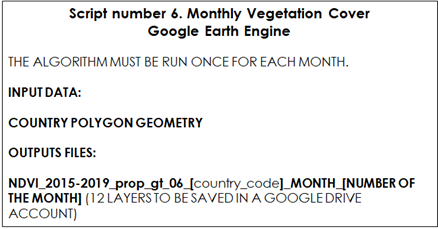
writeRaster(NPP_MIAMI_MEAN_81_00,filename="NPP_MIAMI_MEAN_81-00_MAX.tif",format="GTiff",overwrite=TRUE)9.2.3 Script Number 6. “Monthly_vegetation_cover” vegetation cover from Google Earth Engine.
Script number 6 is a Google Earth Engine script. It is aimed at estimating an average vegetation cover status for each month of the year. Therefore, the script should be run twelve times, modifying the month number each time. It estimates, within a specified time series, the probability for each pixel to present NDVI values greater than a specified threshold, over which the soil is vegetated (for example NDVI > 0.6). The result will vary between 0 and 1. Users may modify the time series and NDVI threshold as desired and according to local knowledge.
Table 9.6. Script Number 6.GEE Monthly Vegetation Cover. Inputs and Outputs
First, the user will need to activate a Google Earth Engine account. To run the Google Earth Engine (GEE) tool, the user will need to copy and paste the script (provided below) into the GEE code editor (central panel, Fig. 9.1).
Figure 9.1 Google Earth Engine code editor
The user will need to draw a polygon that includes the country that is being analyzed, by clicking on “+new layer”. The polygon will contain the country’s boundary or area of interest (Fig. 9.2)
Figure 9.2 Drawing a polygon in Google Earth Engine
The script shall be run twelve times, once for each month of the year. The user will need to specify the month, the name of the output folder and the name of the output raster each time the script is run. The following lines need to be edited:
- Line 10, the month number to be processed, (e.g. for January (1,1,‘month’);
- Line 55, the name of the folder where the output raster file is to be saved (in the Google Drive Account);
- Line 56, the name of the output raster which coincides with the month number that has been run.
//Google Earth Engine
// Monthly Vegetation Cover for Roth C Model
 // Provide a polygon geometry
 // Select the Modis dataset. MOD13A2 is an NDVI product. Modify the number of the month filter for each month from 1 to 12.
 var dataset = ee.ImageCollection('MODIS/006/MOD13A2')
                  .filter(ee.Filter.date('2015-01-01', '2019-12-01'))
                  .filter(ee.Filter.calendarRange(12,12,'month'));
 var ndvi = dataset.select('NDVI');
 // Masks every pixel greater than 0.6 NDVI
var mask06= function(image) {
    var mask = image.select('NDVI').gt(3000);
    return image.updateMask(mask);
  };
 // Apply the mask to the dataset (var ndvi)
var ndvi_06=ndvi.map(mask06);
 // Count the number of times a pixel has an NDVI value greater than 0.6
var ndvi_06_nn=ndvi_06.reduce(ee.Reducer.count());
 // Count the total number of values per pixel
var ndvi_nn=ndvi.reduce(ee.Reducer.count());
 // Calculate the proportion of times the NDVI value is greater than 0.6 per pixel
var prop_cover= ndvi_06_nn.divide(ndvi_nn);
 // Color palette
var ndviVis = {
  min: 0.0,
  max: 1.0,
  palette: [
    'FFFFFF', 'CE7E45', 'DF923D', 'F1B555', 'FCD163', '99B718', '74A901',
    '66A000', '529400', '3E8601', '207401', '056201', '004C00', '023B01',
    '012E01', '011D01', '011301'
 ],
};
 // Clip the map with the country geometry
var Recorte = prop_cover.clip(geometry);
 // Add the map to the visualization google earth engine panel
Map.addLayer(Recorte, ndviVis, 'Country')
 // This code block needs to be modify for each month and allows the user to save the map into a Google drive account
var regionJSON = JSON.stringify(Recorte.getInfo());
Export.image.toDrive({
          image: Recorte.select("NDVI_count"),
          folder: "MAPA_ROTH_C",
          description: 'NDVI_2015-2019_prop_gt_06_CR_MES_01',
          scale: 1000,
          region:geometry,
          maxPixels: 1e9
});
After running the script for each month, the layer must be saved to the Google Drive account. To accomplish this, the user will need to click on the “task” button and then click the “run” button (Fig. 9.3)
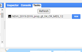
Figure 9.3 Saving the task in GEE.
Once the procedure is completed, the layers should be downloaded from the Google Drive and saved into a local folder
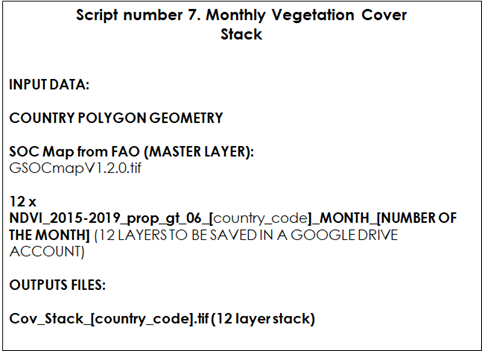
9.2.4 Script Number 7. “Vegetation_Cover_stack.R”
The script number 7 is an R script that uses the monthly vegetation cover layers (0-1 values) created with the GEE script number 6 to create a raster stack. It also linearly rescales the values from “0 to 1” (proportion of vegetated pixels in a time series) to “1 to 0.6” (being 1 = bare soil and 0.6 = full vegetated pixel). This transformation will allow us to use the calculated values as modifying factors of the decomposition rates in the RothC model.
Table 9.6 Script Number 7. Vegetation Cover Stack. Inputs and Outputs.
Once the monthly vegetation cover layers are downloaded from Google Drive, we will generate a stack of those layers. We will first open script number 7 “Vegetation_Cover_stack.R” and the required packages. Then, we will need to open the country polygon vector and set the working directory for the input and the output layers.
library(raster)
library(rgdal)
WD_AOI<-("C:/Training_Material/INPUTS/AOI_POLYGON")
WD_SOC<-("C:/Training_Material/INPUTS/SOC_MAP")
WD_COV<-("C:/Training_Material/INPUTS/INPUTS/COV")


# Open the shapefile of the region/country
setwd(WD_AOI)
AOI<-readOGR("Departamento_Pergamino.shp")
#Open SOC MAP FAO
setwd(WD_SOC)
SOC_MAP_AOI<-raster("SOC_MAP_AOI.tif")
# Open Vegetation Cover layer based only in proportion of NDVI pixels grater than 0.6
setwd(WD_COV)
Cov1<-raster("NDVI_2015-2019_prop_gt03_M01.tif")
Cov1[is.na(Cov1[])] <- 0
Cov1_crop<-crop(Cov1,AOI)
Cov1_mask<-mask(Cov1_crop,AOI)
Cov1_res<-resample(Cov1_mask,SOC_MAP_AOI,method='ngb')
Cov2<-raster("NDVI_2015-2019_prop_gt03_M02.tif")
Cov2[is.na(Cov2[])] <- 0
Cov2_crop<-crop(Cov2,AOI)
Cov2_mask<-mask(Cov2_crop,AOI)
Cov2_res<-resample(Cov2_mask,SOC_MAP_AOI,method='ngb')
Cov3<-raster("NDVI_2015-2019_prop_gt03_M03.tif")
Cov3[is.na(Cov3[])] <- 0
Cov3_crop<-crop(Cov3,AOI)
Cov3_mask<-mask(Cov3_crop,AOI)
Cov3_res<-resample(Cov3_mask,SOC_MAP_AOI,method='ngb')
Cov4<-raster("NDVI_2015-2019_prop_gt03_M04.tif")
Cov4[is.na(Cov4[])] <- 0
Cov4_crop<-crop(Cov4,AOI)
Cov4_mask<-mask(Cov4_crop,AOI)
Cov4_res<-resample(Cov4_mask,SOC_MAP_AOI,method='ngb')
Cov5<-raster("NDVI_2015-2019_prop_gt03_M05.tif")
Cov5[is.na(Cov5[])] <- 0
Cov5_crop<-crop(Cov5,AOI)
Cov5_mask<-mask(Cov5_crop,AOI)
Cov5_res<-resample(Cov5_mask,SOC_MAP_AOI,method='ngb')
Cov6<-raster("NDVI_2015-2019_prop_gt03_M06.tif")
Cov6[is.na(Cov6[])] <- 0
Cov6_crop<-crop(Cov6,AOI)
Cov6_mask<-mask(Cov6_crop,AOI)
Cov6_res<-resample(Cov6_mask,SOC_MAP_AOI,method='ngb')
Cov7<-raster("NDVI_2015-2019_prop_gt03_M07.tif")
Cov7[is.na(Cov7[])] <- 0
Cov7_crop<-crop(Cov7,AOI)
Cov7_mask<-mask(Cov7_crop,AOI)
Cov7_res<-resample(Cov7_mask,SOC_MAP_AOI,method='ngb')
Cov8<-raster("NDVI_2015-2019_prop_gt03_M08.tif")
Cov8[is.na(Cov8[])] <- 0
Cov8_crop<-crop(Cov8,AOI)
Cov8_mask<-mask(Cov8_crop,AOI)
Cov8_res<-resample(Cov8_mask,SOC_MAP_AOI,method='ngb')
Cov9<-raster("NDVI_2015-2019_prop_gt03_M09.tif")
Cov9[is.na(Cov9[])] <- 0
Cov9_crop<-crop(Cov9,AOI)
Cov9_mask<-mask(Cov9_crop,AOI)
Cov9_res<-resample(Cov9_mask,SOC_MAP_AOI,method='ngb')
Cov10<-raster("NDVI_2015-2019_prop_gt03_M10.tif")
Cov10[is.na(Cov10[])] <- 0
Cov10_crop<-crop(Cov10,AOI)
Cov10_mask<-mask(Cov10_crop,AOI)
Cov10_res<-resample(Cov10_mask,SOC_MAP_AOI,method='ngb')
Cov11<-raster("NDVI_2015-2019_prop_gt03_M11.tif")
Cov11[is.na(Cov11[])] <- 0
Cov11_crop<-crop(Cov11,AOI)
Cov11_mask<-mask(Cov11_crop,AOI)
Cov11_res<-resample(Cov11_mask,SOC_MAP_AOI,method='ngb')
Cov12<-raster("NDVI_2015-2019_prop_gt03_M12.tif")
Cov12[is.na(Cov12[])] <- 0
Cov12_crop<-crop(Cov12,AOI)
Cov12_mask<-mask(Cov12_crop,AOI)
Cov12_res<-resample(Cov12_mask,SOC_MAP_AOI,method='ngb')
Stack_Cov<-stack(Cov1_res,Cov2_res,Cov3_res,Cov4_res,Cov5_res,Cov6_res,Cov7_res,Cov8_res,Cov9_res,Cov10_res,Cov11_res,Cov12_res)
# rescale values to 1 if it is bare soil and 0.6 if it is vegetated.
Cov<-((Stack_Cov)*(-0.4))+1
writeRaster(Cov,filename='Cov_stack_AOI.tif',format='GTiff')
Once the monthly vegetation cover layers are downloaded from Google Drive, we will generate a stack of those layers. We will first open script number 7 “Vegetation_Cover_stack.R” and the required packages. Then, we will need to open the country polygon vector and set the working directory for the input and the output layers.
Table 9.8 Script Number 8. Clay Layer from ISRIC. Inputs and Outputs
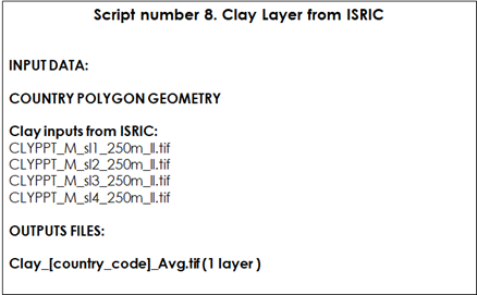
ISRIC clay layers represent the clay content (0-2 micrometer; in g/100g; w%) at four standard depths (Sl1=0-1cm; Sl2=1-5; Sl3=5-15cm; Sl4=15-30 cm) at a 250m resolution. The objective of this script is to aggregate the different layers into one layer by estimating the weighted average of the four depths:
library(raster)
library(rgdal)

WD_AOI<-("C:/Training_Material/INPUTS/AOI_POLYGON")
WD_ISRIC<-("C:/Training_Material/INPUTS/INPUTS/CLAY")
WD_CLAY<-("C:/Training_Material/INPUTS/CLAY")
# Open the shapefile of the region/country
setwd(WD_AOI)
AOI<-readOGR("Departamento_Pergamino.shp")
# Open Clay layers  (ISRIC)
setwd(WD_ISRIC)
Clay1<-raster("CLYPPT_M_sl1_250m_ll_subs.tif")
Clay2<-raster("CLYPPT_M_sl2_250m_ll_subs.tif")
Clay3<-raster("CLYPPT_M_sl3_250m_ll_subs.tif")
Clay4<-raster("CLYPPT_M_sl4_250m_ll_subs.tif")
Clay1_AR<-crop(Clay1,AOI)
Clay2_AR<-crop(Clay2,AOI)
Clay3_AR<-crop(Clay3,AOI)
Clay4_AR<-crop(Clay4,AOI)
# Average of four depths
WeightedAverage<-function(r1,r2,r3,r4){return(r1*(1/30)+r2*(4/30)+r3*(10/30)+r4*(15/30))}
Clay_WA<-overlay(Clay1_AR,Clay2_AR,Clay3_AR,Clay4_AR,fun=WeightedAverage)
Clay_WA_AOI<-mask(Clay_WA,AOI)
setwd(WD_CLAY)
writeRaster(Clay_WA_AOI,filename="Clay_WA_AOI.tif",format='GTiff')
9.3 Preparing the land use layer
The land use layer is one of the most important layers in the process, as it defines the target areas and production systems to be modeled. The land use layer will be needed:
- to account for major land use changes during the 2000-2020 period;
- to obtain the DPM/RPM ratios required in the RothC model ( See Chapter 4);
- to define the modeling units/target points where the model is to be run (agricultural lands in 2020).
Each modeling phase will require specific land use layers. For the ‘spin up’ phase, users should use a representative land use layer for the period 1980-2000 (e.g. land use layer as in year 2000), or best available land use layer. For the ‘warm-up’ phase, users can use year to year land use layers (2000 to 2020), or a representative land use layer for the period, depending on the available information. The ‘warm-up’ land use layer accounts for year to year changes in the land use during the period (for example a pixel that changes from forest to cropland). The script will need a stack of land use layers, one layer for each year of the warm up phase. If the user does not want to model changes in the land use layer over the warm up phase, or information is not available, the same land use layer for each year can be used over the warm-up phase. For the ‘forward’ phase, the latest best available land use layer should be used.
As a minimum, the last available land use data at 1x1 km resolution shall be defined. The predominant land use category in each cell of the 1x1 km grid shall be selected if finer resolutions are available.
The land use classes can be derived from land cover classes from different national, regional or global datasets which best correlate with national land use. The land use layers are used in the three modelling phases to generate a decomposition rate DR layer (generated through scripts 10, 11, and 12, See sections 9.8-9.10), that represents the above mentioned DPM/RPM ratios for the different land use classes. In scripts 10,11 and 12, default DPM/RPM values are assigned to each FAO Global Land Cover (GLC-SHARE) class (See Table 6.1 Chapter 6; Section 6.7; and scripts 10,11 and 12). For more information on this classification refer to FAO (2014) and to the FAO Land and Water site: http://www.fao.org/land-water/land/land-governance/land-resources-planning-toolbox/category/details/en/c/1036355/
Thus, land cover classes obtained from different datasets (e.g. European Space Agency - ESA) need to be re-classified into FAO land cover classes in a Geotiff format if the scripts 10,11 and 12 are to be run with the default land classes and DPM/RPM ratios provided with the training material.
In this section, we provide a script to transform ESA land use cover classes to FAO land use classes (script 9), which can be used as a model to convert and use classes from other datasets. Users can however modify the DPM/RPM default values (See Table 6.1, Chapter 6) based on local knowledge and available information, create additional land use classes or disaggregate the FAO land use classes, and assign DPM/RPM ratios to those new classes by modifying the provided scripts. Users are encouraged to leverage available local knowledge and data to produce the most accurate SOCseq maps possible. With this in mind, if more detailed land use maps, i.e. containing information about the types of cropping systems present, and local data on the DPM/RPM for the specific land use types are easily accessible, the provided script should be edited accordingly.
Finally, the land use layer is also needed to define the target points where the three phases of the protocol will be run. In section 9.7 we provide a Qgis model to generate the target points from the land use layer. Defining the target points out of the land use layer will allow us to run the model just in the pixels with the land use classes of interest.
Depending on whether yearly land use layers are available for the forward phase, this technical manual contains alternative scripts both for the data preparation phase (Scripts 9_Land_Use_ESA_to_FAO_classes_LUsim.R and 11_WARM_UP_STACK_V5_LUsim.R) and the modelling phase (Script 14_ROTH_C_WARM_UP_UNC_v3_LUsim.R). Figure illustrates the script sequence to be followed depending on whether yearly land use change layers are available for the warm up phase.
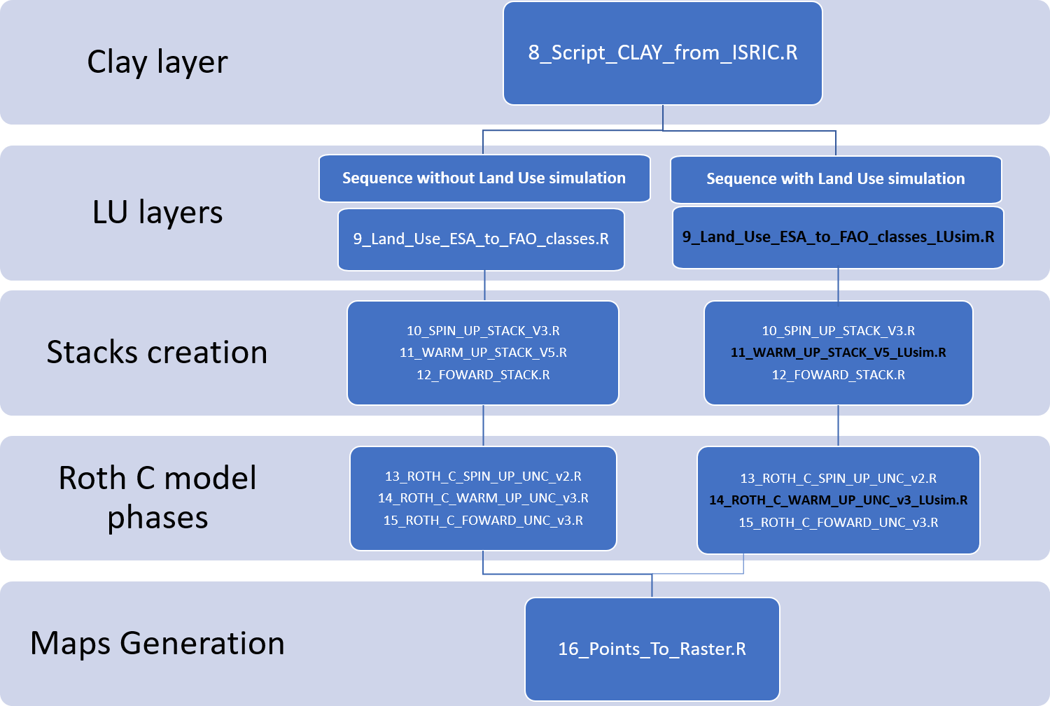 ***
***
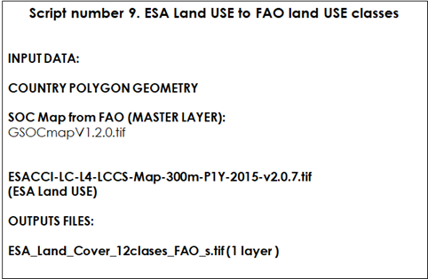
9.3.1 Script Number 9 “Land_Use_ESA_to_FAO_classes.R” No land use change
Script number 9 transforms the ESA (European Space Agency 2015; 300 m resolution; ESA CCI Land cover website) land cover classes to the FAO land use classes. This script can be modified to be used with any other land use dataset.
Table 9.9 Script Number 9. ESA Land Use to FAO classes. Inputs and Outputs
First, we will need to open the R packages, open the shapefile of the region/country to be modelled, and open the land use/land cover data set to be re-classified into FAO land use classes:
library(raster)
library(rgdal)
WD_AOI<-("C:/Training_Material/INPUTS/AOI_POLYGON")
WD_LU<-("C:/Training_Material/INPUTS/LAND_USE")
WD_SOC<-("C:/Training_Material/INPUTS/SOC_MAP")
# Open the shapefile of the region/country
setwd(WD_AOI)
AOI<-readOGR("Departamento_Pergamino.shp")
# Open Land Use Layer (ESA)
setwd(WD_LU)
ESA_LU<-raster("ESACCI-LC-L4-LCCS-Map-300m-P1Y-2015-v2.0.7_subs.tif")
plot(ESA_LU)
# Cut the LU layer by the country polygon
ESA_LU_AOI<-crop(ESA_LU,AOI)
plot(ESA_LU_AOI)
# Reclassify ESA LAND USE to FAO LAND USE classes
#     0 = 0   No Data
#   190 = 1 Artificial
#   10 11 20 30 40 = 2 Croplands
#   130 = 3 Grassland
#   50 60 61 62 70 71 72 80 81 82 90 100 110 = 4 Tree Covered
#   120 121 122= 5 Shrubs Covered
#   160 180 = 6 Herbaceous vegetation flooded
#   170 = 7 Mangroves
#   150 151 152 153= 8 Sparse Vegetation
#   200 201 202 = 9 Baresoil
#   220 = 10 Snow and Glaciers
#   210 = 11 Waterbodies
#   12 = 12 Treecrops
#   20 = 13 Paddy fields(rice/ flooded crops)
# Reclassify matrix. "Is" to "become"
is<-c(0,190,10,11,20,30,40,130,50,60,61,62,70,71,72,80,81,82,90,100,110,120,121,122,160,180,170,150,151,152,153,200,201,202,220,210,12)
become<-c(0,1,2,2,2,2,2,3,4,4,4,4,4,4,4,4,4,4,4,4,4,5,5,5,6,6,7,8,8,8,8,9,9,9,10,11,12)
recMat<-matrix(c(is,become),ncol=2,nrow=37)
# Reclassify
ESA_FAO <- reclassify(ESA_LU_AOI, recMat)
# Resample to SOC map layer extent and resolution
setwd(WD_SOC)
SOC_MAP_AOI<-raster("SOC_MAP_AOI.tif")
ESA_FAO_res<-resample(ESA_FAO,SOC_MAP_AOI,method='ngb')
ESA_FAO_mask<-mask(ESA_FAO_res,SOC_MAP_AOI)
# Save Land Use raster
setwd(WD_LU)
writeRaster(ESA_FAO_mask,filename="ESA_Land_Cover_12clases_FAO_AOI.tif",format='GTiff')
9.3.2 Script Number 9 “Land_Use_ESA_to_FAO_classes_LUsim.R” Land use change simulation
Script number 9 transforms the ESA (European Space Agency 2000 to 2018; 300 m resolution; ESA CCI Land cover website) land cover classes to the FAO land use classes. This script allows for the preparation of a stack with yearly land use layers to simulate land use change during the warm up phase.
#DATE: 11-02-2021

# MSc Ing Agr Luciano E Di Paolo
# Dr Ing Agr Guillermo E Peralta

#### Prepare Land Use layer

rm(list = ls())

library(raster)
library(rgdal)

WD_AOI<-("C:/TRAINING_MATERIALS_GSOCseq_MAPS_12-11-2020/INPUTS/AOI_POLYGON")

WD_LU<-("C:/TRAINING_MATERIALS_GSOCseq_MAPS_12-11-2020/INPUTS/LAND_USE")

WD_SOC<-("C:/TRAINING_MATERIALS_GSOCseq_MAPS_12-11-2020/INPUTS/SOC_MAP")

# Open the shapefile of the region/country

setwd(WD_AOI)
AOI<-readOGR("Departamento_Pergamino.shp") # change for your own Area of interest

# Open Land Use Layer (ESA)

setwd(WD_LU)
ESA_LU<-stack("LU_stack_ESA_2001-2018.tif")
plot(ESA_LU[[1]])

# Cut the LU layer by the country polygon

ESA_LU_AOI<-crop(ESA_LU,AOI)

plot(ESA_LU_AOI[[1:4]])

# Reclassify ESA LAND USE to FAO LAND USE classes

#   0 = 0     No Data
#   190 = 1 Artificial
#   10 11 30 40 = 2 Croplands
#   130 = 3 Grassland
#   50 60 61 62 70 71 72 80 81 82 90 100 110 = 4 Tree Covered
#   120 121 122= 5 Shrubs Covered
#   160 180 = 6 Herbaceous vegetation flooded
#   170 = 7 Mangroves
#   150 151 152 153= 8 Sparse Vegetation
#   200 201 202 = 9 Baresoil
#   220 = 10 Snow and Glaciers
#   210 = 11 Waterbodies
#   12  = 12 Treecrops
# 20 = 13 Paddy fields(rice/ flooded crops)

# Create a reclassification matrix. "Is" to "become"

is<-c(0,190,10,11,30,40,130,50,60,61,62,70,71,72,80,81,82,90,100,110,120,121,122,160,180,
170,150,151,152,153,200,201,202,220,210,12,20)

become<-c(0,1,2,2,2,2,3,4,4,4,4,4,4,4,4,4,4,4,4,4,5,5,5,6,6,7,8,8,8,8,9,9,9,10,11,12,13)

recMat<-matrix(c(is,become),ncol=2,nrow=37)

# Reclassify

ESA_FAO <- reclassify(ESA_LU_AOI, recMat)

# Resample to SOC map layer extent and resolution
setwd(WD_SOC)
SOC_MAP_AOI<-raster("SOC_MAP_AOI.tif") # change for your own SOC MAP

ESA_FAO_res<-resample(ESA_FAO,SOC_MAP_AOI,method='ngb')
ESA_FAO_mask<-mask(ESA_FAO_res,SOC_MAP_AOI)

# Save Land Use raster
setwd(WD_LU)
writeRaster(ESA_FAO_mask,filename="ESA_Land_Cover_12clases_FAO_Stack_AOI.tif",format='GTiff',overwrite=TRUE)

# We save separately the land use from 2018 to perform the target's points creation
writeRaster(ESA_FAO_mask[[18]],filename="ESA_Land_Cover_12clases_FAO_2018_AOI.tif",format='GTiff',overwrite=TRUE)
Table 9.9 Script Number 9. ESA Land Use to FAO classes. Inputs and Outputs
9.4 Harmonization of soil, climate and vegetation layers.
Once all soil, climate, vegetation and land use layers are created, they need to be harmonized in order to run the model. The harmonization of layers consists of three steps. First, if the model is to be run for an entire country, layers need to be harmonized to the extents of the country boundaries (country polygon layer extents). Second, a resampling process is required in order to match the spatial resolution to the master layer (SOC FAO layer). Finally, a masking process is required to cut the layer with the vector polygon boundaries. After the harmonization of all layers, we will generate a raster stack of all layers needed to run the model. The harmonization/stacking process will be performed three times (scripts 10,11,12), one for each modelling phase.
9.4.1 Script Number 10. “SPIN_UP_STACK.v3.R”
Script number 10 is intended to harmonize all layers needed to complete phase 1 (long spin-up) of the spatial RothC model. The result of this script is a simple raster stack which contains all the data to perform the spin-up phase. To generate the stack we will need the SOC FAO layer (master layer), the clay layer (from script number 8), the three climate stacks (from script number 1), the land use layer (from script number 9), and the vegetation cover stack (from script number 7).
Table 9.10 Script Number 10. Stack Layers for SPIN UP phase. Inputs and Outputs
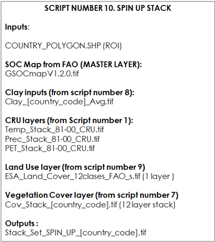
First, we will open the required R-packages and a shapefile (polygon) which represents the country boundary. In the script below we will be using an example but when running it (AR), the user will have to replace the file according to the target country. The user can also modify the names of the variables inside the script. However, as these variables will only exist inside the script, it is not necessary.
#### Prepare the layers for the SPIN UP process of the Roth C Model.
rm(list = ls())
library(raster)
library(rgdal)
WD_AOI<-("C:/Training_Material/INPUTS/AOI_POLYGON")
WD_SOC<-("C:/Training_Material/INPUTS/SOC_MAP")
WD_CLAY<-("C:/Training_Material/INPUTS/CLAY")
WD_CLIM<-("C:/Training_Material/INPUTS/CRU_LAYERS")
WD_LU<-("C:/Training_Material/INPUTS/LAND_USE")
WD_COV<-("C:/Training_Material/INPUTS/COV")
WD_STACK<-("C:/Training_Material/INPUTS/STACK")
# Open the shapefile of the region/country
setwd(WD_AOI)
AOI<-readOGR("Departamento_Pergamino.shp")

The second step is to load the latest version of FAO Soil Organic Carbon map layer (Master Layer), created in script number 0.
#Open SOC MAP FAO
setwd(WD_SOC)
SOC_MAP_AOI<-raster("SOC_MAP_AOI.tif")
 Next, we will open the clay content layer (from script number 8):
# Open Clay layer
setwd(WD_CLAY)
Clay_WA_AOI<-raster("Clay_WA_AOI.tif")
Clay_WA_AOI_res<-resample(Clay_WA_AOI,SOC_MAP_AOI,method='bilinear')
Clay_AR_Avg<-crop(Clay_AR_Avg,AR)
Clay_AR_Avg<-mask(Clay_AR_Avg,AR)
Clay_AR_Avg_res<-resample(Clay_AR_Avg,SOC_MAP_AR,method='bilinear')
Next, we will open the climate raster layers (generated in script number 1).  These layers come from the CRU database, but the user can choose local layers if desired, as long as they match the arrangement and format needed for running the model.
#Open Precipitation layer
setwd(WD_CLIM)
PREC<-stack("Prec_Stack_81-00_CRU.tif")
PREC_AOI<-crop(PREC,AOI)
PREC_AOI<-resample(PREC_AOI,SOC_MAP_AOI)
PREC_AOI<-mask(PREC_AOI,AOI)
PREC_AOI<-stack(PREC_AOI)
#Open Temperatures layer (CRU https://crudata.uea.ac.uk/cru/data/hrg/)
TEMP<-stack("Temp_Stack_81-00_CRU.tif")
TEMP_AOI<-crop(TEMP,AOI)
TEMP_AOI<-resample(TEMP_AOI,SOC_MAP_AOI)
TEMP_AOI<-mask(TEMP_AOI,AOI)
TEMP_AOI<-stack(TEMP_AOI)
#Open Potential Evapotranspiration layer (CRU https://crudata.uea.ac.uk/cru/data/hrg/)
PET<-stack("PET_Stack_81-00_CRU.tif")
PET_AOI<-crop(PET,AOI)
PET_AOI<-resample(PET_AOI,SOC_MAP_AOI)
PET_AOI<-mask(PET_AOI,AOI)
PET_AOI<-stack(PET_AOI)
Next, we will open, resample and mask the land use raster layer to be used in the spin up phase (representative 1980-2000 period).  In this example we will use the ESA land used reclassified into FAO land use classes (script 9)
# OPen Land Use layer reclassify to FAO classes
# 0 No Data
# 1 Artificial
# 2 Croplands
# 3 Grassland
# 4 Tree Covered
# 5 Shrubs Covered
# 6 Herbaceous vegetation flooded
# 7 Mangroves
# 8 Sparse Vegetation
# 9 Baresoil
# 10 Snow and Glaciers
# 11 Waterbodies
# 12 TreeCrops
# 13 Paddy fields
setwd(WD_LU)
LU_AOI<-raster("ESA_Land_Cover_12clases_FAO_AOI.tif")
Then, we will open the vegetation cover layers (created in script number 7):
# Open Vegetation Cover layer
setwd(WD_COV)
Cov_AOI<-stack('Cov_stack_AOI.tif')
The script then creates a DR layer (DPM/RPM ratio). Here the DR layer is derived from the Land use layer, assigning default DPM/RPM ratios to each FAO land cover class (See Table 9.13). Users can modify these ratios according to local expertise and available local information.
# Use Land use layer to convert it to DR layer
#DPM/RPM (decomplosable vs resistant plant material)
#(1) Most agricultural crops and improved grassland and tree crops 1.44
#(2) Unimproved grassland and schrub 0.67
#(3) Deciduous and tropical woodland 0.25
DR<-(LU_AOI==2 | LU_AOI==12| LU_AOI==13)*1.44+ (LU_AOI==4)*0.25 + (LU_AOI==3 | LU_AOI==5 | LU_AOI==6 | LU_AOI==8)*0.67
 Finally, we will create a stack with all the raster layers that have been prepared.
 # STACK all layers
Stack_Set_AOI<-stack(SOC_MAP_AOI,Clay_WA_AOI_res,TEMP_AOI,PREC_AOI,PET_AOI,DR,LU_AOI,Cov_AOI)
setwd(WD_STACK)
writeRaster(Stack_Set_AOI,filename=("Stack_Set_SPIN_UP_AOI.tif"),format="GTiff")
9.4.2 Script Number 11. “WARM_UP_STACK_V5.R” No Land use change
Script number 11 is intended to harmonize all layers required to run the phase 2 (WARM UP) of the spatial RothC model. The result of this script is a simple raster stack which contains most of the layers needed for the warm-up phase. To generate the stack we will need the latest version of SOC FAO layer (master layer), the clay layer (from script number 8), land use layers (from script number 9), a land use stack (one land use layer per year), a vegetation cover stack (from script number 7) and the NPP stack (from script number 4). The climate layers and the NPP mean are additional layers that will be needed in the WARM UP phase but will not be part of this stack because of the final size of the output file.
Table 9.11 Script Number 11. Stack layers for Warm Up phase. Inputs and Outputs
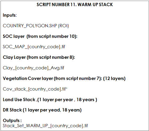
First, we will load the packages, set the number of years of the warmup phase and set the directories of each layer. Then we will open the country vector polygon boundaries:
rm(list = ls())
library(raster)
library(rgdal)
# Set the number of years of the warm up
nWUP<-18
WD_AOI<-("C:/Training_Material/INPUTS/AOI_POLYGON")

WD_SOC<-("C:/Training_Material/INPUTS/SOC_MAP")
WD_CLAY<-("C:/Training_Material/INPUTS/INPUTS/CLAY")
WD_CLIM<-("C:/Training_Material/INPUTS/CRU_LAYERS")
WD_LU<-("C:/Training_Material/INPUTS/LAND_USE")
WD_COV<-("C:/Training_Material/INPUTS/COV")
WD_STACK<-("C:/Training_Material/INPUTS/STACK")
WD_NPP<-("C:/Training_Material/INPUTS/NPP")
# Open the shapefile of the region/country
setwd(WD_AOI)
AOI<-readOGR("Departamento_Pergamino.shp")
Then, we will open the harmonized FAO GSOCmap of the country created in script number 0:
#Open SOC MAP
setwd(WD_SOC)
SOC_MAP_AOI<-raster("SOC_MAP_AOI.tif")
Then we will open the clay layer created in script number 8:
 # Open Clay layers  (ISRIC)
setwd(WD_CLAY)
Clay_WA_AOI<-raster("Clay_WA_AOI.tif")
Clay_WA_AOI_res<-resample(Clay_WA_AOI,SOC_MAP_AOI,method='bilinear')
Then, we will open the Land Use layers required for the warm up phase (2000-2020). In this example we used the ESA land use (2015) reclassified into to the FAO land use classes.
# OPen Land Use layer (ESA)
setwd(WD_LU)
LU_AOI<-raster("ESA_Land_Cover_12clases_FAO_AOI.tif")
We will then open the vegetation cover layer previously created in the script number 7:
# Open Vegetation Cover layer
setwd(WD_COV)
Cov_AOI<-stack('Cov_stack_AOI.tif')
If year to year land use layers are available for the warm up phase (2000-2020), we will open the Land Use stack of the annual land use layers. If annual land use layers are not available, we will just replicate a representative land use layer for the warm-up phase, as previously loaded.
# Open Land Use Stack , One Land use layer for each year (in this example we use the same LU for the 18/20 year #period set previously in the nWUP variable
 LU_Stack <-stack(replicate(nWUP, LU_AOI))
Then, we will create a “DR” stack layer, one DR layer per year of the WARM UP phase.
# Create DR Layer from LU layer (ESA land use , 14 classes)
#DPM/RPM (decomposable vs resistant plant material)
#(1) Most agricultural crops and improved grassland or tree crops 1.44
#(2) Unimproved grassland and shrub 0.67
#(3) Deciduous and tropical woodland 0.25
DR<-(LU_AOI==2 | LU_AOI==12| LU_AOI==13)*1.44+ (LU_AOI==4)*0.25 + (LU_AOI==3 | LU_AOI==5 | LU_AOI==6 | LU_AOI==8)*0.67
DR_Stack<-LU_Stack
for (i in 1:nlayers(LU_Stack)){
DR_Stack[[i]]<-(LU_Stack[[i]]==2 | LU_Stack[[i]]==12)*1.44+ (LU_Stack[[i]]==4)*0.25 + (LU_Stack[[i]]==3 | LU_Stack[[i]]==5 | LU_Stack[[i]]==6 | LU_Stack[[i]]==8)*0.67
}
Finally, we will run the rest of the code and save the raster stack containing all the necessary layers to run the ‘warm up’ phase.
# STACK all layers
Stack_Set_AOI<-stack(SOC_MAP_AOI,Clay_WA_AOI_res,Cov_AOI,LU_Stack,DR_Stack)
setwd(WD_STACK)
writeRaster(Stack_Set_AOI,filename=("Stack_Set_WARM_UP_AOI.tif"),format="GTiff")
9.4.3 Script Number 11. WARM_UP_STACK_V5_LUsim.R Land use change simulation
The following script is to be used if yearly land use layers to simulate land use change are available. This script uses the output from script numer 9 Land_Use_ESA_to_FAO_classes_LUsim.R
#DATE 11-2-2021
# ADD NPP_MIN AND NPP_MAX TO THE STACK TO CALCULATE UNCERTAINTIES

# MSc Ing Agr Luciano E Di Paolo
# Dr Ing Agr Guillermo E Peralta


#### Prepare the layers for the WARM UP Roth C Model.

rm(list = ls())

library(raster)
library(rgdal)

# Set the number of years of the warm up
nWUP<-18

WD_AOI<-("C:/TRAINING_MATERIALS_GSOCseq_MAPS_12-11-2020/INPUTS/AOI_POLYGON")

WD_SOC<-("C:/TRAINING_MATERIALS_GSOCseq_MAPS_12-11-2020/INPUTS/SOC_MAP")

WD_CLAY<-("C:/TRAINING_MATERIALS_GSOCseq_MAPS_12-11-2020/INPUTS/CLAY")

WD_CLIM<-("C:/TRAINING_MATERIALS_GSOCseq_MAPS_12-11-2020/INPUTS/CRU_LAYERS")

WD_LU<-("C:/TRAINING_MATERIALS_GSOCseq_MAPS_12-11-2020/INPUTS/LAND_USE")

WD_COV<-("C:/TRAINING_MATERIALS_GSOCseq_MAPS_12-11-2020/INPUTS/COV")

WD_STACK<-("C:/TRAINING_MATERIALS_GSOCseq_MAPS_12-11-2020/INPUTS/STACK")

WD_NPP<-("C:/TRAINING_MATERIALS_GSOCseq_MAPS_12-11-2020/INPUTS/NPP")


# Open the shapefile of the region/country
setwd(WD_AOI)
AOI<-readOGR("Departamento_Pergamino.shp") # change the AOI

#Open SOC MAP

setwd(WD_SOC)
SOC_MAP_AOI<-raster("SOC_MAP_AOI.tif") # change the SOC_MAP

# Open Clay layers  (ISRIC)

setwd(WD_CLAY)

Clay_WA_AOI<-raster("Clay_WA_AOI.tif")

Clay_WA_AOI_res<-resample(Clay_WA_AOI,SOC_MAP_AOI,method='bilinear')

# OPen Land Use layer (ESA)

# 0 No Data
# 1 Artificial
# 2 Croplands
# 3 Grassland
# 4 Tree Covered
# 5 Shrubs Covered
# 6 Herbaceous vegetation flooded
# 7 Mangroves
# 8 Sparse Vegetation
# 9 Baresoil
# 10 Snow and Glaciers
# 11 Waterbodies
# 12 TreeCrops
# 13 Paddy fields


setwd(WD_LU)
LU_AOI<-stack("ESA_Land_Cover_12clases_FAO_Stack_AOI.tif")

# Open Vegetation Cover layer

setwd(WD_COV)

Cov_AOI<-stack('Cov_stack_AOI.tif')

# Open Land Use Stack , One Land use layer for each year (in this example we use the same LU for the 18 year period

#LU_Stack <-stack(replicate(nWUP, LU_AOI))
#LU_Stack <-stack(ESA[2001:2015],2015,2015,2015)
LU_Stack<-LU_AOI

# Convert LU layer  to DR layer (ESA land use , 14 classes)

#DPM/RPM (decomplosable vs resistant plant material)
#(1) Most agricultural crops and improved grassland or tree crops 1.44
#(2) Unimproved grassland and schrub 0.67
#(3) Deciduous and tropical woodland 0.25

#DR<-(LU_AOI==2 | LU_AOI==12 | LU_AOI==13)*1.44+ (LU_AOI==4)*0.25 + (LU_AOI==3 | LU_AOI==5 | LU_AOI==6 | LU_AOI==8)*0.67

DR_Stack<-LU_Stack

for (i in 1:nlayers(LU_Stack)){
DR_Stack[[i]]<-(LU_Stack[[i]]==2 | LU_Stack[[i]]==12 | LU_Stack[[i]]==13)*1.44+ (LU_Stack[[i]]==4)*0.25 + (LU_Stack[[i]]==3 | LU_Stack[[i]]==5 | LU_Stack[[i]]==6 | LU_Stack[[i]]==8)*0.67
}

# STACK all layers

Stack_Set_AOI<-stack(SOC_MAP_AOI,Clay_WA_AOI_res,Cov_AOI,LU_Stack,DR_Stack)

setwd(WD_STACK)
writeRaster(Stack_Set_AOI,filename=("Stack_Set_WARM_UP_AOI.tif"),format="GTiff",overwrite=TRUE)
9.4.4 Script Number 12. “FORWARD_STACK.R”
Script number 12 harmonizes all layers needed to run phase 3 (forward) of the spatial Roth C model. The result of the script is a simple raster stack which contains the layers needed to perform the forward phase. To generate the stack we will need the SOC FAO layer (master layer), the clay layer (from script number 8), the three climate stacks required for the forward phase (from script number 2), the land use layer or the forward phase (from script number 9), and the vegetation cover stack (from script number 7).
Table 9.12 Script Number 12. Stack layers for forward phase. Inputs and Outputs.
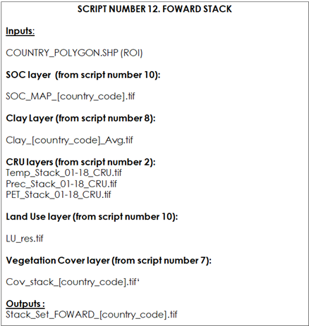
First, we will load the packages, set path to the files directories and open the country vector polygon boundaries.
9.4.4.1 Prepare the layers for the FOWARD Mode Roth C Model.
rm(list = ls())
library(raster)
library(rgdal)

WD_AOI<-("C:/Training_Material/INPUTS/AOI_POLYGON")
WD_SOC<-("C:/Training_Material/INPUTS/SOC_MAP")
WD_CLAY<-("C:/Training_Material/INPUTS/CLAY")
WD_CLIM<-("C:/Training_Material/INPUTS/CRU_LAYERS")
WD_LU<-("C:/Training_Material/INPUTS/LAND_USE")
WD_COV<-("C:/Training_Material/INPUTS/COV")
WD_STACK<-("C:/Training_Material/INPUTS/STACK")
# Open the shapefile of the region/country
setwd(WD_AOI)
AOI<-readOGR("Departamento_Pergamino.shp")
Then, we will open the SOC layer and the clay layer.
#Open SOC MAP
setwd(WD_SOC)
SOC_MAP_AOI<-raster("SOC_MAP_AOI.tif")
# Open Clay layers  (ISRIC)
setwd(WD_CLAY)
Clay_WA_AOI<-raster("Clay_WA_AOI.tif")
Clay_WA_AOI_res<-resample(Clay_WA_AOI,SOC_MAP_AOI,method='bilinear')

Then we will open the 2000-2020 average climate layers created (as the one created in script number 2)
#Open Precipitation layer (CRU https://crudata.uea.ac.uk/cru/data/hrg/)
setwd(WD_CLIM)
PREC<-stack("Prec_Stack_01-18_CRU.tif")
PREC_AOI<-crop(PREC,AOI)
PREC_AOI<-resample(PREC_AOI,SOC_MAP_AOI)
PREC_AOI<-mask(PREC_AOI,AOI)
PREC_AOI<-stack(PREC_AOI)
#Open Temperatures layer (CRU https://crudata.uea.ac.uk/cru/data/hrg/)
TEMP<-stack("Temp_Stack_01-18_CRU.tif")
TEMP_AOI<-crop(TEMP,AOI)
TEMP_AOI<-resample(TEMP_AOI,SOC_MAP_AOI)
TEMP_AOI<-mask(TEMP_AOI,AOI)
TEMP_AOI<-stack(TEMP_AOI)
#Open Potential Evapotranspiration layer (CRU https://crudata.uea.ac.uk/cru/data/hrg/)
PET<-stack("PET_Stack_01-18_CRU.tif")
PET_AOI<-crop(PET,AOI)
PET_AOI<-resample(PET_AOI,SOC_MAP_AOI)
PET_AOI<-mask(PET_AOI,AOI)
PET_AOI<-stack(PET_AOI)
Then, we will open the land use layer (latest available year) created in script number 10.
setwd(WD_LU)
LU_AOI<-raster("ESA_Land_Cover_12clases_FAO_AOI.tif")
Then, we will open the vegetation cover layer created in script number 7.
# Open Vegetation Cover
setwd(WD_COV)
Cov_AOI<-stack('Cov_stack_AOI.tif')
As in the previous scripts, this script creates a DR layer (DPM/RPM ratio), assigning default DPM/RPM ratios to each FAO land cover class (See Table 9.13). Users can modify these ratios according to local expertise and available local information.
# Open Land use layer and convert it to DR layer (mod 12 , 14 classes)
#DPM/RPM (decomplosable vs resistant plant material...como se divide los C inputs)
#(1) Most agricultural crops and improved grassland or tree crops 1.44
#(2) Unimproved grassland and schrub 0.67
#(3) Deciduous and tropical woodland 0.25
DR<-(LU_AOI==2 | LU_AOI==12| LU_AOI==13)*1.44+ (LU_AOI==4)*0.25 + (LU_AOI==3 | LU_AOI==5 | LU_AOI==6 | LU_AOI==8)*0.67
We will create a stack for the forward modelling phase. We will have to define the filename and save the output stack.
# STACK all layers
Stack_Set_AR<-stack(SOC_MAP_AOI,Clay_WA_AOI_res,TEMP_AOI,PREC_AOI,PET_AOI,DR,LU_AOI,Cov_AOI)
setwd(WD_STACK)
writeRaster(Stack_Set_AR,filename=("Stack_Set_FOWARD.tif"),format="GTiff")
9.5 Defining target points to run the model
At this point we have three raster stacks for the different modelling phases. We need to create the points where those simulations will be run in order to accelerate the modelling process. These points will be the center of the pixels of the master layer (GSOCmap layer, script number 7). Later, we will convert the points containing the modelling output values back to a raster layer format.
9.5.1 QGIS Procedure number 1 (model)
We will need the land use data of each pixel (we already corregistered the land use layer with the master layer at script number 7). Then we will use the land use layer of the country to generate the points. For this, we can use a QGIS model to create target points.
Table 9.13 QGis procedure number 1. Create target points to run the model. Inputs and Outputs
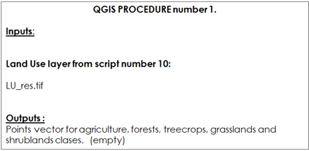
We will open the Qgis, then go to the processing toolbox and click on the “open existing model” button. We will have to search for the model in the provided folder, called “4_Points_country”. We will have to load the model called “Qgis_Procedure_number_1.model3”. Once this is done, we can run the model from the processing toolbox.
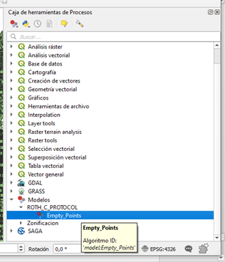
Figure 9.4 Processing toolbox in Qgis
We will click the Empty_Points button and a window will pop up. We will select the Land use layer created in script number 10 (already resampled to match the extent and pixel size of the GSOCmap), set the path and the name of the output file, and click on the Execute button.
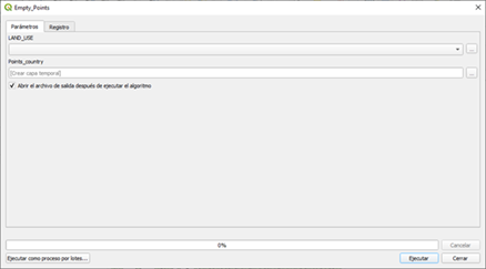
Figure 9.5 Qgis Window to edit the points generated.
This process will create vector points. Each point will be created in the centroid of each pixel of the land use layer. This vector will contain no fields. The scripts to run the model for each phase (SPIN_UP, WARM_UP, forward) will attach all the necessary data from the stacks (scripts number 10, 11 and 12) to each point.