 Soil Sampling Design
Chapter 5 Stratified Simple Random Sampling
Stratified simple random sampling is a technique where the study area is divided into different groups or strata based on certain environmental traits and a number of random samples are taken from within each group. One of the primary advantages of stratified sampling is its ability to capture the diversity within a population by making sure each group is represented. It can provide a more accurate reflection of the entire population compared to random sampling, especially when the groups are distinct and have unique qualities. This approach is particularly beneficial when certain subgroups within the population are specifically noteworthy. It also allows for more precise estimates with a smaller total sample size compared to simple random choice. Stratified sampling presents some disadvantages. Achieving effective categories requires a proper definition and delineation of the initial information to create the strata. The classification of the environmental information into categories and ensuring fair portrayal of each can be intricate and time–taking and mislabeling elements into an improper group can lead to skewed outcomes.
5.1 General Procedure
The creation of a stratified simple random sampling design involves the identification of relevant features describing the environmental diversity in the area (soil and landcover are the environmental variables generally used to define strata), delineation of the strata, determination of the number of samples to distribute to each stratum, followed by random sampling within it. By identifying relevant classes, combining them to define strata and allocating an appropriate number of samples to each stratum, a representative sample can be obtained. Random sampling within each stratum helps to ensure that the sample is unbiased and provides a fair representation of the overall conditions in the area.
The first question is about how many samples must be retrieved from each strata. The sampling scheme starts with the definition of the total number of samples to collect. In this case, the determination of the sample size is a complex and highly variable process based, among others, on the specific goals of the study, the variability of environmental proxies, the statistical requirements for accuracy and confidence, as well as additional considerations such as accessibility, costs and available resources. The optimal number of samples can be determined following the method proposed in Chapter 2 of this manual. The number of samples within each stratum is calculated using an area–weighted approach taking into account the relative area of each stratum. The sampling design in this section must also comply with the following requirements:
- All sampling strata must have a minimum size of 100 hectares.
- All sampling strata must be represented by at least 2 samples.
This sampling process ensures the representativeness of the environmental combinations present across the area while maintaining an efficient and feasible field sampling campaign.
5.1.1 Strata creation
We must determine the kind of information that will be used to construct the strata. In this manual, we present a simple procedure to build strata based on data from two environmental layers: soil groups and landcover classification data. The information should be provided in the form of vector shapefiles with associated information databases. The data on both sets often comprises a large number of categories, that would lead to a very large number of strata. Thus, it is desirable to make an effort of aggregating similar categories within each input data set, to reduce, as much as possible, the number of categories while still capturing the most of the valuable variability in the area.
The fist step is to set–up the RStudio environment and load the required packages:
We must define the number of samples to distribute in the sampling design and the soil and landcover information layers to build the strata. We also define a BOUNDARY parameter to account for a reduction of the sampling area according to a certain area using predefined bounding–box, that can be also here defined.
We proceed with the calculation of soil groups. In this example, soil information is stored in the field SRG. We have analysed the extent to which the information in this field can be synthesized to eliminate redundancy when creating the strata. 1.
The results are shown in 5.1
## Plot aggregated soil classes
map <- leaflet(leafletOptions(minZoom = 8)) %>%
addTiles()
mv <- mapview(soil["RSG"], alpha=0, homebutton=T, layer.name = "soils", map=map)
mv@mapFigure 5.1: Plot of the soil classes
#ggplot() + geom_sf(data=soil, aes(fill = factor(RSG)))A similar procedure is performed on the landcover dataset.
Figure 5.2 shows the landcover classes to build the strata.
# Plot map with the land cover information
map <- leaflet() %>%
addTiles()
mv <- mapview(lc["landcover"], alpha=0, homebutton=T, layer.name = "Landcover", map=map)
mv@mapFigure 5.2: Plot of the landcover classes
#ggplot() + geom_sf(data=lc, aes(fill = factor(landcover)))To create the soil–landcover strata we must combine both classified datasets.
# Combine soil and landcover layers
sf_use_s2(FALSE)
soil_lc <- st_intersection(st_make_valid(soil), st_make_valid(lc))
soil_lc$soil_lc <- paste0(soil_lc$RSG, "_", soil_lc$landcover)
soil_lc <- soil_lc %>% dplyr::select(soil_lc, geometry)Finally, to comply with the initial requirements of the sampling design, we calculate the areas of each polygon, delete all features with extent lesser than 100 has.
# Select by Area. Convert to area to ha and select polygons with more than 100 has
soil_lc$area <- st_area(soil_lc)/10000
soil_lc$area <- as.vector(soil_lc$area)
soil_lc <- soil_lc %>%
group_by(soil_lc) %>%
mutate(area = sum(area))
soil_lc <- soil_lc[soil_lc$area > 100,]
# Replace blank spaces with underscore symbol to keep names uniform
soil_lc$soil_lc <- str_replace_all(soil_lc$soil_lc, " ", "_")
# Create a column of strata numeric codes
soil_lc$code <- as.character(as.numeric(as.factor(soil_lc$soil_lc))) # Write final sampling strata map
st_write(soil_lc, paste0(results.path,"strata.shp"), delete_dsn = TRUE)The final strata map is shown in Figure 5.3.
# Plot final map of stratum
map <- leaflet(options = leafletOptions(minZoom = 8.3)) %>%
addTiles()
mv <- mapview(soil_lc["soil_lc"], alpha=0, homebutton=T, layer.name = "Strata", map=map)
mv@mapFigure 5.3: Plot of strata
5.2 Stratified random sampling
This example demonstrates how to establish a stratified random sampling approach within the previously defined strata polygons. The allocation of sample points is proportionate to the stratum areas, with the condition that each stratum must contain a minimum of 2 samples. The determination of sampling points, referred to as 'target points', is made during the initial phase of the sampling design and takes into consideration factors such as the area to be sampled, budget constraints and available personnel. Additionally, a set number of 'replacement points' must be designated to act as substitutes for ‘target points’ in cases where some of the original target points cannot be accessed or sampled. These ‘replacement points’ are systematically indexed, with each index indicating which ‘target point’ it serves as a substitute for.
Results are shown in Figure 5.4.
map <- leaflet(options = leafletOptions(minZoom = 8.3)) %>%
addTiles()
mv <- mapview(soil_lc["soil_lc"], alpha=0, homebutton=T, layer.name = "Strata") +
mapview(sf::st_as_sf(z), zcol = 'type', color = "white", col.regions = c('royalblue', 'tomato'), cex=3, legend = TRUE,layer.name = "Samples")
mv@mapFigure 5.4: Plot of strata and random target and replacement points
5.3 Stratified simple random sampling for large areas
The implementation of a stratified simple random sampling, along with target and replacement points, can present operating difficulties when dealing with areas of significant size and with locations that are hard to reach. To address this issue, the sampling approach can be modified by excluding areas with limited accessibility.
This modification can streamline fieldwork operations and establish a feasible sampling method while still retaining the essence of the stratified simple random sampling framework. By excluding areas with limited accessibility, the sampling design can be adjusted to ensure a more practical and effective approach to data collection.
Delineation of sampling accessibility: The sampling area can be further limited based on accessibility considerations. Areas with very limited accessibility, defined as regions located more than 1 kilometre away from a main road or access path, may be excluded from sampling areas. To accomplish this, a map of main roads and paths can be used to establish a sampling buffer that includes areas within a 1–kilometre buffer around the road infrastructures. This exclusion helps to eliminate the most remote and challenging–to–access areas. An additional layer of accessibility information can be incorporated based on population distribution in the country, considering that, if population is present, there is a high change that points in the surroundings can be accessible for sampling. In this case, populated nuclei are vectorized into points and a 250–meter buffer is then generated around each point. These resulting areas can be then added to the 1–kilometre buffer around the roads, which collectively defined the final sampling area.
Substitution of replacement points with replacement areas in close proximity to the target points: The sampling design presented before included designated replacement points to serve as substitutes for each target point in the case that it would be inaccessible during fieldwork. However, this approach presented challenges, particularly for large areas, as the replacement point could be located far from the target point, resulting in significant logistical efforts. This limitation posed a risk of delays in completing the sampling campaign within the allocated time frame. To address this challenge, an alternative strategy is to replace the idea of replacement points with replacement areas situated in the immediate vicinity of the target point. The replacement area for each target point is now confined within a 500–meter buffer surrounding the target and falls within the same sampling stratum. This approach concentrates sampling and replacement activities within a specific geographic area, streamlining the overall process. By reducing the need for extensive travel, this method enhances efficiency and facilitates sample collection. Figure 2 illustrates the distribution of sampling points and replacement areas for visualization.
Additional area exclusion: Some areas can be identified as not suitable for sampling purposes. This is the case of certain natural protected areas, conflict regions presenting risks for field operators, etc. These areas must be identified masked at an initial stage of the design to exclude them from the sampling strata.
The procedure is the same as that previously presented, with the difference that buffers and exclusion areas must be masked–out from the strata map before performing the random sampling.
# Compute replacement sampling areas -----
# Load strata
soil_lc <- st_read(paste0(results.path,"strata.shp"))
# Read sampling. points from previous step
z <- st_read(paste0(results.path,"strat_randm_samples.shp"))
z <- z[z$type=="Target",]
# Define buffer of 500 meters (coordinate system must be in metric base)
buf.samples <- st_buffer(z, dist=distance.buffer)
# Intersect buffers
samples_buffer = st_intersection(soil_lc, buf.samples)
samples_buffer <- samples_buffer[samples_buffer$type=="Target",]
samples_buffer <- samples_buffer[samples_buffer$soil_lc==samples_buffer$group,]
# Save Sampling areas
st_write(samples_buffer, paste0('../soil_sampling/JAM/replacement_areas_', samples.buffer, '.shp'), delete_dsn = TRUE)
# Write target points only
targets <- z[z$type=="Target",]
st_write(targets, '../soil_sampling/JAM/sampling_points_TAR.shp', delete_dsn = TRUE)5.4 Stratified simple regular sampling
The procedure for creating a stratified simple regular sampling design is identical to that presented for stratified simple random sampling, with the only distinction that the locations of the sampling points are distributed in a regular spatial grid. This transformation is achieved by changing the method from ‘random’ to ‘regular’ in the spatSample functions within the script above.
# Export data to Shapefile ----
# Write sampling points to shp
writeVector(z, paste0(results.path,"sampling_points.shp"), overwrite=TRUE)
# Check whether the number of initial target points equals the final target points
n;nrow(z[z$type=="Target",]) map <- leaflet(options = leafletOptions(minZoom = 8.3)) %>%
addTiles()
mv <- mapview(soil_lc["soil_lc"], alpha=0, homebutton=T, layer.name = "Strata") +
mapview(sf::st_as_sf(z), zcol = 'type', color = "white", col.regions = c('royalblue', 'tomato'), cex=3, legend = TRUE,layer.name = "Samples")
mv@mapFigure 5.5: Plot of strata and regular sampling points
5.5 Simple Random Sampling based on a stratified raster
Finally, it is also possible to create a stratified area weighted random sampling using raster strata. The procedure involves the creation of the strata as a raster file and implement a random sampling using the frequencies of the strata as a guideline for distribution of the samples proportionally to their frequencies. This method is easily implemented using the package ‘sgsR’ (Goodbody, Coops and Queinnec, 2023).
#strata <- st_read(paste0(results.path,"strata.shp"),quiet = TRUE)
strata <- soil_lc
strata$code <- as.integer(strata$code)
# Create stratification raster
strata <- rast(st_rasterize(strata["code"],st_as_stars(st_bbox(strata), nx = 250, ny = 250)))
names(strata) <- "strata"
strata <- crop(strata, nghe, mask=TRUE)
# Create stratified simple random sampling
target <- sample_strat(
sraster = strata,
nSamp = n
)
target$type <- "target"Figure 5.6 show the histogram of frequencies of samples over the strata categories respectively.
# Histogram of frequencies
calculate_representation(
sraster = strata,
existing = target,
drop=0,
plot = TRUE
)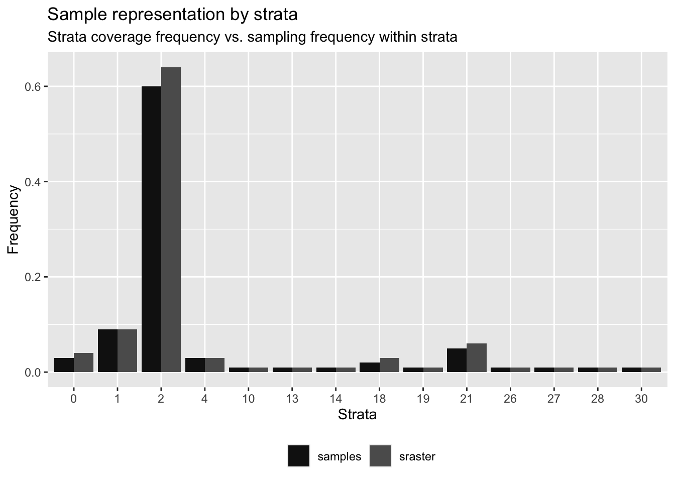
Figure 5.6: Frequencies of strata and random target samples
## # A tibble: 14 × 6
## strata srasterFreq sampleFreq diffFreq nSamp need
## <dbl> <dbl> <dbl> <dbl> <int> <dbl>
## 1 0 0.04 0.03 -0.01 9 2
## 2 1 0.09 0.09 0 24 1
## 3 2 0.64 0.6 -0.0400 161 10
## 4 4 0.03 0.03 0 8 1
## 5 10 0.01 0.01 0 3 0
## 6 13 0.01 0.01 0 3 0
## 7 14 0.01 0.01 0 2 1
## 8 18 0.03 0.02 -0.01 6 3
## 9 19 0.01 0.01 0 3 0
## 10 21 0.06 0.05 -0.0100 14 3
## 11 26 0.01 0.01 0 2 1
## 12 27 0.01 0.01 0 2 1
## 13 28 0.01 0.01 0 3 0
## 14 30 0.01 0.01 0 4 -1 # Add index by strata
target <- target %>%
st_as_sf() %>%
dplyr::group_by(strata) %>%
dplyr::mutate(order = seq_along(strata),
ID = paste0(strata, ".", order)) %>%
vect()The construction of replacement points is straightforward by creating a new stratified set of samples on the same strata. In this case, the sample size has been incremented 3 times to create 3 replacement points for each target point.
# Create replacement points
replacement <- sample_strat(
sraster = strata,
nSamp = nrow(target)*3
)
replacement$type <- "replacement" # Histogram of frequencies
calculate_representation(
sraster = strata,
existing = replacement,
drop=0,
plot = TRUE
)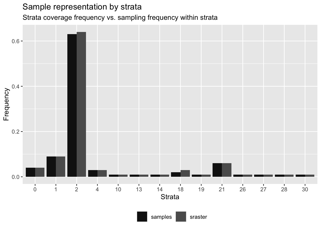
Figure 5.7: Frequencies of strata and random replacement samples
## # A tibble: 14 × 6
## strata srasterFreq sampleFreq diffFreq nSamp need
## <dbl> <dbl> <dbl> <dbl> <int> <dbl>
## 1 0 0.04 0.04 0 29 4
## 2 1 0.09 0.09 0 76 -2
## 3 2 0.64 0.63 -0.0100 515 6
## 4 4 0.03 0.03 0 27 -2
## 5 10 0.01 0.01 0 10 -1
## 6 13 0.01 0.01 0 10 -1
## 7 14 0.01 0.01 0 7 2
## 8 18 0.03 0.02 -0.01 20 5
## 9 19 0.01 0.01 0 8 1
## 10 21 0.06 0.06 0 46 3
## 11 26 0.01 0.01 0 6 3
## 12 27 0.01 0.01 0 8 1
## 13 28 0.01 0.01 0 10 -1
## 14 30 0.01 0.01 0 11 -2 # Add index by strata
replacement <- replacement %>%
st_as_sf() %>%
dplyr::group_by(strata) %>%
dplyr::mutate(order = seq_along(strata),
ID = paste0(strata, ".", order)) %>%
vect()
# Merge target and replacement points in a single object
sampling.points <- rbind(target,replacement)Figures 5.7 and 5.8 show the frequencies of replacement samples over the strata categories and the distribution of target and replacement samples respectively.
# Plot samples over strata
map <- leaflet(options = leafletOptions(minZoom = 8.3)) %>%
addTiles()
mv <- mapview(st_as_stars(strata),homebutton=T, layer.name = "Strata") +
mapview(sampling.points, zcol = 'type', color = "white", col.regions = c('royalblue', 'tomato'), cex=3, legend = TRUE,layer.name = "Samples")
mv@mapFigure 5.8: Plot of raster strata and sampling points
The resulting target and replacement points can finally be stored as shapefiles.
## Export to shapefile
writeVector(sampling.points,
paste0(results.path,"pts_raster.shp"), overwrite=TRUE)References
This exploratory work is a prerequisite and must be adapted specifically to each soil and landcover dataset↩︎