 Soil Sampling Design
Chapter 3 Evaluating Soil Legacy Data Sampling for DSM
Modelling techniques in Digital Soil Mapping involve the use of sampling point soil data, with its associated soil properties database, and a number of environmental covariates that will be used to ascertain the relationships of soil properties and the environment to then generalize the findings to locations where no samples have been compiled.
In soil sampling design, a crucial issue is to determine both the locations and the number of the samples to be compiled. In an optimal situation, soil sample database should adequately cover all the environmental diversity space in the study area with a frequency relative to the extent of the diversity in the environmental covariates.
When dealing with legacy soil data, a question that arises is if the data is representative of the environmental diversity within the study area. In this Chapter we present a method to answer this question and to build an alternative how many samples can be retrieved to cover the same environmental space as the existing soil data. The method follows the main findings in (Malone, Minansy and Brungard, 2019) and developed as {R} scripts.
We adapted the original scripts to make use of vector '.shp' and raster '.tif' files, as these are data formats commonly used by GIS analysts and in which both soil and environmental data is often stored. We also made some changes in order to simplify the number of R packages and to avoid the use of deprecated packages as it appears in the original code.
3.1 Data Preparation
We must load the required packages and data for the analyses. We make use of the packages sp and terra to manipulate spatial data, clhs for Conditioned Latin Hypercube Sampling, entropy to compute Kullback–Leibler (KL) divergence indexes, tripack for Delaunay triangulation and manipulate for interactive plotting within RStudio. Ensure that all these packages are installed in your system before the execution of the script.
We define the working directory to the directory in which the actual file is located and load the soil legacy sampling points and the environmental rasters from the data folder. To avoid the definition of each environmental covariate, we first retrieve all files with the .tif extension and then create a SpatRaster object with all of them in a row.
  ## Set working directory to source file location
    setwd(dirname(rstudioapi::getActiveDocumentContext()$path))
Here we define a number of variables that will be used during the exercises in this manual. They include the path to raster and shp files, aggregation and disaggregation factors, and buffer distances to define potential sampling areas from sampling points. These variables are later described at the appropriate section in the manual.
The original covariates are cropped to match the extent of a smaller area, the Nghe An province in this exercise, to simplify the computation time. Then, covariates are transformed by Principal Component Analysis to uncorrelated Principal Component scores. This ensures the use of a lower amount of raster data avoiding multicollinearity in the original covariates. We select the Principal Component rasters that capture 99% of the variability in the dataset.
  ## Load soil legacy point data and environmental covariates
  # Read Spatial data covariates as rasters with terra
  cov.dat <-  list.files(raster.path, pattern = "tif$",  recursive = TRUE, full.names = TRUE)
  cov.dat <- terra::rast(cov.dat) # SpatRaster from terra
  # Aggregate stack to simplify data rasters for calculations
  cov.dat <- aggregate(cov.dat, fact=agg.factor, fun="mean")

  # Load shape of district
  nghe <- sf::st_read(file.path(paste0(shp.path,"/Nghe_An.shp")),quiet=TRUE)

  # Crop covariates on administrative boundary
  cov.dat <- crop(cov.dat, nghe, mask=TRUE)

  # Transform raster information with PCA
  pca <- raster_pca(cov.dat)

  # Get SpatRaster layers
  cov.dat <- pca$PCA

  # Subset rasters to main PC (var. explained <=0.99)
  n_comps <- first(which(pca$summaryPCA[3,]>0.99))
  cov.dat <- pca$PCA[[1:n_comps]]

  # convert to dataframe
  cov.dat.df <- as.data.frame(cov.dat)

  # Load legacy soil data
  p.dat <- terra::vect(file.path(paste0(shp.path,"/legacy_soils.shp")))
Figure 3.1 shows the PCA-transformed raster layers used in the analyses.
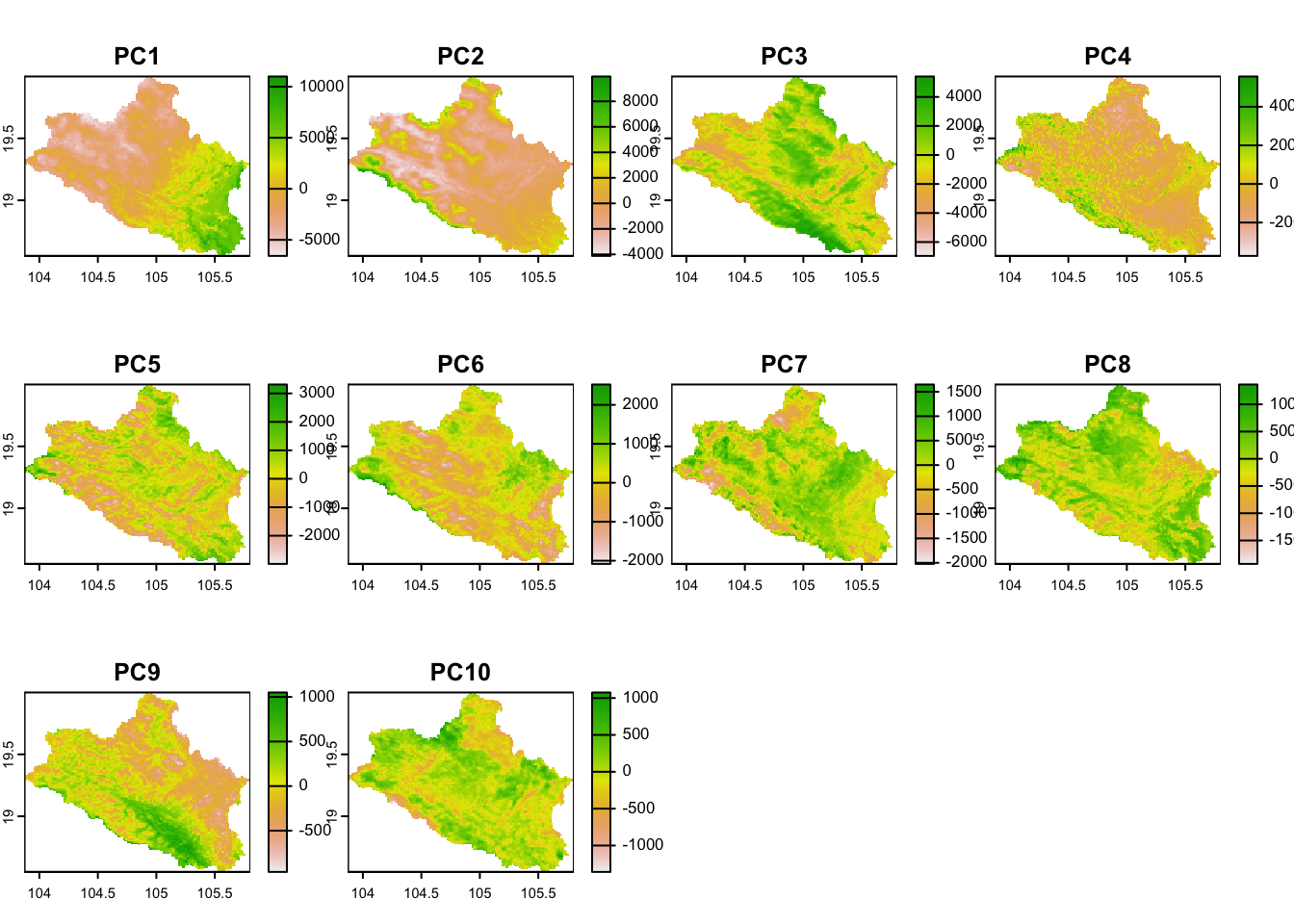
Figure 3.1: Covariates
3.2 Representativeness of the Legacy Soil Data
The next step involves determining the distributions of environmental values in the soil samples data and comparing them with the existing distributions of each environmental variable to assess the representativeness of the existing soil samples in the environmental space.
The comparison of distributions is performed using the Kullback–Leibler divergence (KL) distance, a measure used to quantify the difference between two probability distributions. KL–divergence compares an ‘objective’ or reference probability distribution (in this case, the distribution of covariates in the complete covariate space – P) with a ‘model’ or approximate probability distribution (the values of covariates in the soil samples – Q). The main idea is to determine how much information is lost when Q is used to approximate P. In other words, KL–divergence measures how much the Q distribution deviates from the P distribution. KL–divergence approaches 0 as the two distributions have identical quantities of information.
To create a dataset with the values of the environmental parameters at the locations of the soil samples, we cross-reference soil and environmental data.
First, we calculate a ‘n–matrix’ with the values of the covariates, dividing their values into ‘n’ bins according to an equal–probability distribution. Each bin captures the environmental variability within its interval in the total distribution. In this exercise, ‘n’ equals to 25. The result is a 26×4 matrix, where the rows represent the upper and lower limit of the bin (26 thresholds are required to represent 25 bins), and the columns correspond to the number of variables used as environmental proxies.
  ## Variability matrix in the covariates
    # Define Number of bins
      nb <- 25
      #quantile matrix (of the covariate data)
      q.mat <- matrix(NA, nrow=(nb+1), ncol= nlyr(cov.dat))
      j=1
      for (i in 1:nlyr(cov.dat)){ #note the index start here
      #get a quantile matrix together of the covariates
        ran1 <- minmax(cov.dat[[i]])[2] - minmax(cov.dat[[i]])[1]
        step1 <- ran1/nb
        q.mat[,j] <- seq(minmax(cov.dat[[i]])[1], to = minmax(cov.dat[[i]])[2], by =step1)
        j<- j+1}
From this matrix, we compute the hypercube matrix of covariates in the whole covariate space.
## Hypercube of "objective" distribution (P) – covariates
  # Convert SpatRaster to dataframe for calculations
      cov.mat <- matrix(1, nrow = nb, ncol = ncol(q.mat))
      cov.dat.mx <- as.matrix(cov.dat.df)
      for (i in 1:nrow(cov.dat.mx)) {
        for (j in 1:ncol(cov.dat.mx)) {
          dd <- cov.dat.mx[[i, j]]

          if (!is.na(dd)) {
            for (k in 1:nb) {
              kl <- q.mat[k, j]
              ku <- q.mat[k + 1, j]

              if (dd >= kl && dd <= ku) {
                cov.mat[k, j] <- cov.mat[k, j] + 1
              }
            }
          }
        }
      }
Te, we calculate the hypercube matrix of covariates in the sample space.
## Sample data hypercube
      h.mat <- matrix(1, nrow = nb, ncol = ncol(q.mat))
      for (i in 1:nrow(p.dat_I.df)) {
        for (j in 1:ncol(p.dat_I.df)) {
          dd <- p.dat_I.df[i, j]

          if (!is.na(dd)) {
            for (k in 1:nb) {
              kl <- q.mat[k, j]
              ku <- q.mat[k + 1, j]

              if (dd >= kl && dd <= ku) {
                h.mat[k, j] <- h.mat[k, j] + 1
              }
            }
          }
        }
}- KL–divergence
We calculate the KL–divergence to measure how much the distribution of covariates in the sample space (Q) deviates from the distribution of covariates in the complete study area space (P).
  ## Compare covariate distributions in P and Q with Kullback–Leibler (KL) divergence
      kl.index <-c()
      for(i in 1:ncol(cov.dat.df)){
        kl <-    KL.empirical(c(cov.mat[,i]), c(h.mat[,i]))
        kl.index <- c(kl.index,kl)
        klo <-  mean(kl.index)
      }
      #print(kl.index) # KL divergences of each covariate
      #print(klo) # KL divergence in the existing soil samples
The KL–divergence is always greater than or equal to zero, and reaches its minimum value (zero) only when P and Q are identical. Thus, lower values of KL–divergence indicate a better match between both the sample and the study area spaces, suggesting that the sample space provides a fair representation of the environmental conditions in the study area.
In this case, the KL–divergence value is 0.181, which quantifies the amount of environmental variability in the study area captured by the legacy samples.
- Percent of representativeness in relation to the overall environmental conditions
Finally, we can assess the extent to which our legacy soil dataset represents the existing environmental conditions in the study area. We calculate the proportion of pixels in the study area that would fall within the convex hull polygon delineated based on the environmental conditions found only at the locations of the soil legacy data. The convex hull polygon is created using a Principal Component transformation of the data in the soil legacy dataset, utilizing the outer limits of the scores of the points projected onto the two main components (Fig. 3.2).
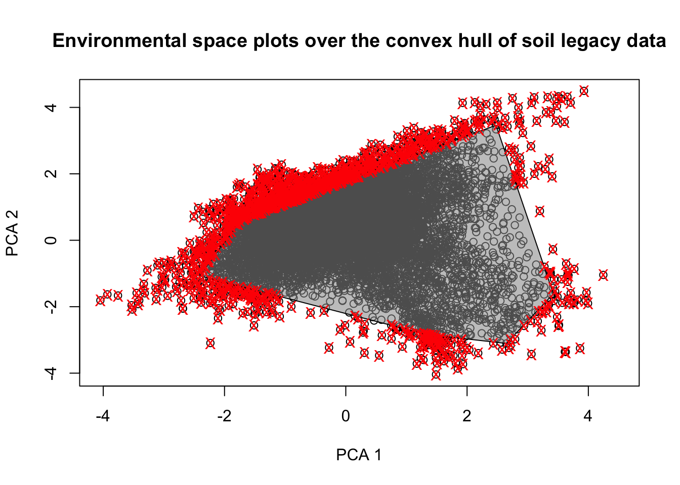
Figure 3.2: PCA plot of the covariate
This indicates that 90.3% of the existing conditions in the study area are encompassed within the convex hull delineated using the data from the soil samples. This percentage shows the level of adequacy of the legacy data for DSM in the area.