 Soil Sampling Design
Chapter 6 Conditioned Latin Hypercube Sampling
Conditioned Latin Hypercube Sampling (cLHS) is an advanced statistical method used for sampling multidimensional data developed within the context of digital Soil Mapping. It’s an extension of the basic Latin Hypercube Sampling (LHS) technique, a statistical method for generating a distribution of samples of a random variable. The main advantage of LHS over simple random sampling is its ability to ensure that the entire range of the auxiliary variables are explored. It divides the range of each variable into intervals of equal probability and samples each interval.
The term ‘conditioned’ refers to the way the sampling is adapted or conditioned based on specific requirements or constraints. It often involves conditioning the sampling process on one or more additional variables or criteria. This helps in generating samples that are not just representative in terms of the range of values, but also in terms of their relationships or distributions. cLHS is particularly useful for sampling from multivariate data, where there are multiple interrelated variables as it occurs in soil surveys. The main advantage of cLHS is its efficiency in sampling and its ability to better capture the structure and relationships within the data, compared to simpler sampling methods and ensures that the samples are representative not just of the range of each variable, but also of their interrelations. Detailed information on cLHS can be found in (Minasny and McBratney, 2006).
In this technical manual, we primarily utilize the R implementation of cLHS provided by the sgsR package (Goodbody et al., 2023). This implementation is based on the work of (Roudier et al., 2011), also available on CRAN as the clhs package. The latter is specifically employed for some of the analyses presented in this document.
6.1 cLHS Design
As for stratified sampling, the creation target points from a conditioned Latin Hypercube Sampling design involves the identification of the relevant features describing the environmental diversity in the area. In this case, the environmental parameters are incorporated in the form of raster covariates. The determination of the number of samples in the design is also required. This step can be calculated following the information already provided in this manual.
With the minimum sampling size of 182 calculated before, we can conduct conditioned Latin Hypercube Sampling design for the area in the example using the R packages 'sgsR' and 'cLHS' available at CRAN.
  # Path to rasters
  raster.path <- "data/rasters/"
  # Path to shapes
  shp.path <- "data/shapes/"
  # Path to results
  results.path <- "data/results/"
  # Path to additional data
  other.path <- "data/other/"

  # Aggregation factor for up-scaling raster covariates (optional)
  agg.factor = 10
  # Buffer distance for replacement areas (clhs)
  D <- 1000 # Buffer distance to calculate replacement areas
  # Define the minimum sample size. By default it uses the value calculated previously
  #minimum_n <- minimum_n
We use the rasters of as covariates, which we trim by the administrative boundary of the ‘Nghe An’ province as an example to speed up the calculations in the exercise. The rasters are loaded as a raster stack, masked, and subjected to PCA transformation to reduce collinearity in the dataset. The PCA components that capture 99% of the variability in the data are retained as representatives of the environmental diversity in the area. Rasters of elevation and slope are kept separately for further analyses. A shapefile of roads is also loaded to account for the sampling cost associated with walking distances from roads.
  # Read Spatial data covariates as rasters with terra
  cov.dat <-  list.files(raster.path, pattern = "tif$",  recursive = TRUE, full.names = TRUE)
  cov.dat <- terra::rast(cov.dat) # SpatRaster from terra
  # Load shape of district
  nghe <- sf::st_read(file.path(paste0(shp.path,"/Nghe_An.shp")),quiet=TRUE)

  # Crop covariates on administrative boundary
  cov.dat <- crop(cov.dat, nghe, mask=TRUE)
  # Store elevation and slope separately
  elevation <- cov.dat$dtm_elevation_250m
  slope <- cov.dat$dtm_slope_250m
  # Load roads
  roads <-  sf::st_read(file.path(paste0(shp.path,"/roads.shp")),quiet=TRUE)
  roads <-  st_intersection(roads, nghe)
# Simplify raster information with PCA
pca <- raster_pca(cov.dat)
# Get SpatRaster layers
cov.dat <- pca$PCA
# Subset rasters
n_comps <- first(which(pca$summaryPCA[3,]>0.99)) # Select PC explaining >=99%
cov.dat <- pca$PCA[[1:n_comps]]
# Remove pca stack
rm(pca)
# Aggregate stack to simplify data rasters for calculations
# cov.dat <- aggregate(cov.dat, fact=10, fun="mean") # Plot of covariates
plot(cov.dat)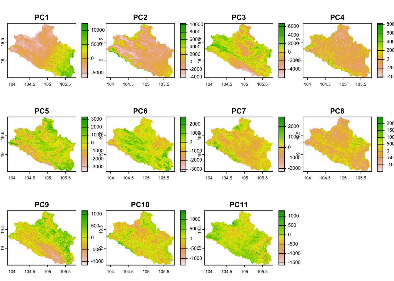
Figure 6.1: Covariates
The distribution of the sampling points is obtained using the 'sample_clhs'function together with the stack of raster covariates and the minimum number of samples calculated in the previous Section. The function uses a number of iterations for the Metropolis–Hastings annealing process, with a default of 10000, to determine the optimal location of samples that account for a maximum of information on the raster covariates.
  # Distribute sampling points with clhs
  pts <-  sample_clhs(cov.dat, nSamp = 100, iter = 10000, progress = FALSE, simple = FALSE)
The distribution of points is shown in Figure 6.2.
  # Plot cLHS samples on map
  plot(cov.dat[[1]], main="cLHS samples")
  points(pts, col="red", pch = 1)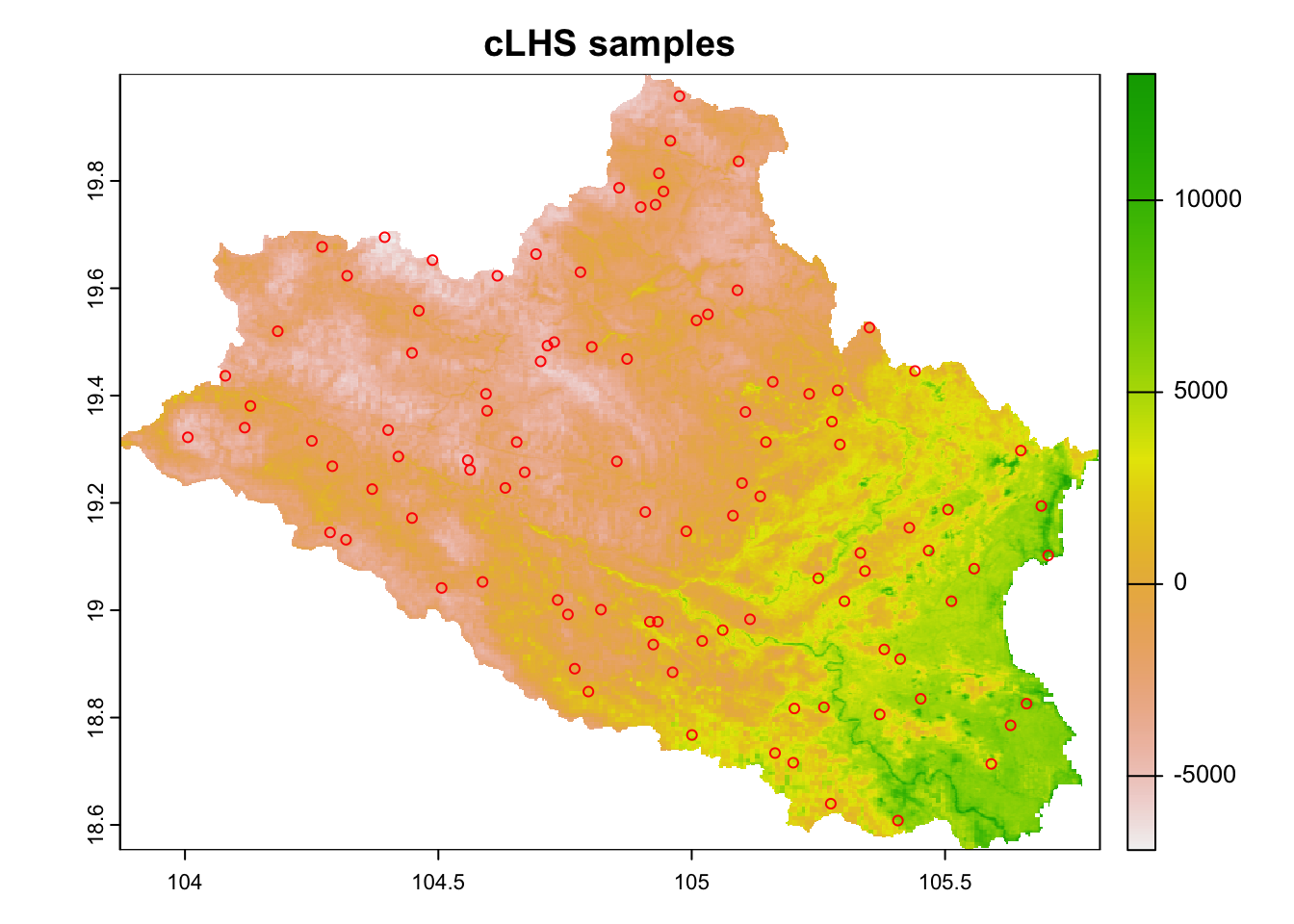
Figure 6.2: Distribution of cLHS sampling points in the study area
6.2 Including existing legacy data in a cLHS sampling design
In situations where there are legacy soil data samples available, it would be interesting to include them in the cLHS design to increase the diversity of covariates and avoid oversampling for some conditions. In this cases, the ancillary data can be included in the design as additional points to the 'sample_clhs' function.
  # Create an artificial random legacy dataset of 50 samples over the study area as an example
  legacy.data <- sample_srs( raster = cov.dat, nSamp = 50)

  # Calculate clhs 100 points plus locations of legacy data
  res <-  sample_clhs(cov.dat, nSamp = 150, existing=legacy.data, iter = 10000, progress = FALSE)
Figure 6.3 shows the distribution of the created cLHS samples, which also include the position of the original legacy soil data points.
  # Plot points
  plot(cov.dat[[1]], main="cLHS samples (blue circles) and legacy samples (red diamonds)")
  points(res, col="navy", pch = 1)
  points(res[res$type=="existing",], col="red", pch = 5, cex=2)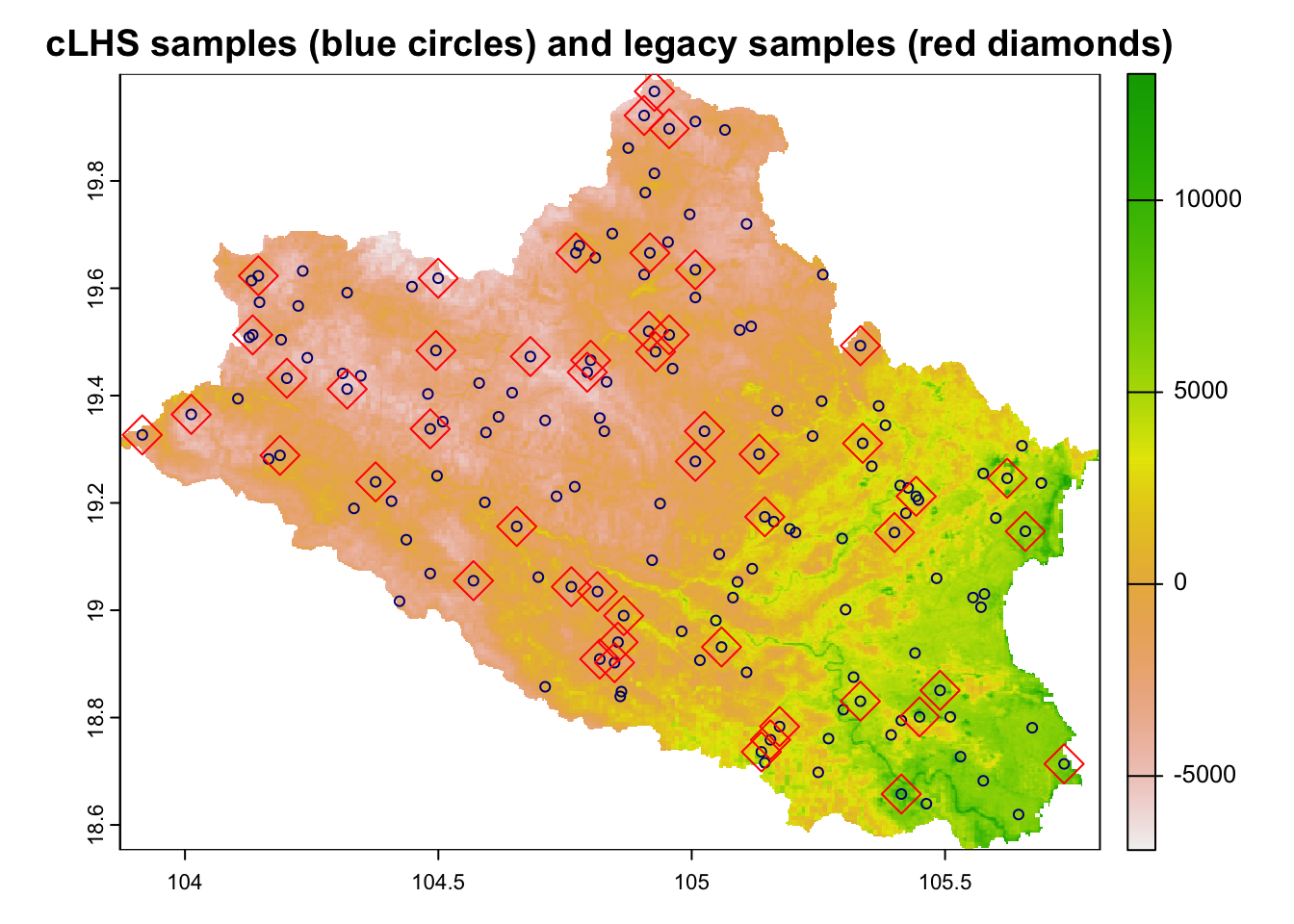
Figure 6.3: cLHS sampling points with legacy data
6.3 Working with large raster data
The 'sample_clhs' function samples the covariates in the raster stack in order to determine the optimal location of samples that best represent the environmental conditions in the area. In the case of working with large raster sets, the process can be highly computing demanding since all pixels in the raster stack are used in the process. There are two simple methods to avoid this constraint:
- Aggregation of covariates: The quickest solution is to aggregate the covariates in the raster stack to a lower pixel resolution. This is directly performed using the
'aggregate'function from the'terra'package. In case that the raster stack has discrete layers (factor data), the corresponding layers has to be aggregated separately using either the ‘min’ or ‘max’ functions to avoid corruption of the data and the results added later to the data of continuous raster layers.
    # Aggregation of covariates by a factor of 10.
    # The original grid resolution is up-scaled using the mean value of the pixels in the grid
    cov.dat2 <- aggregate(cov.dat, fact=10, fun="mean")
    # Create clhs samples upon the resampled rasters
    resampled.clhs <- sample_clhs(cov.dat2, nSamp = 150, iter = 10000, progress = FALSE)
# Plot the points over the 1st raster
plot(cov.dat2[[1]], main="cLHS samples")
points(resampled.clhs , col="red", pch = 1)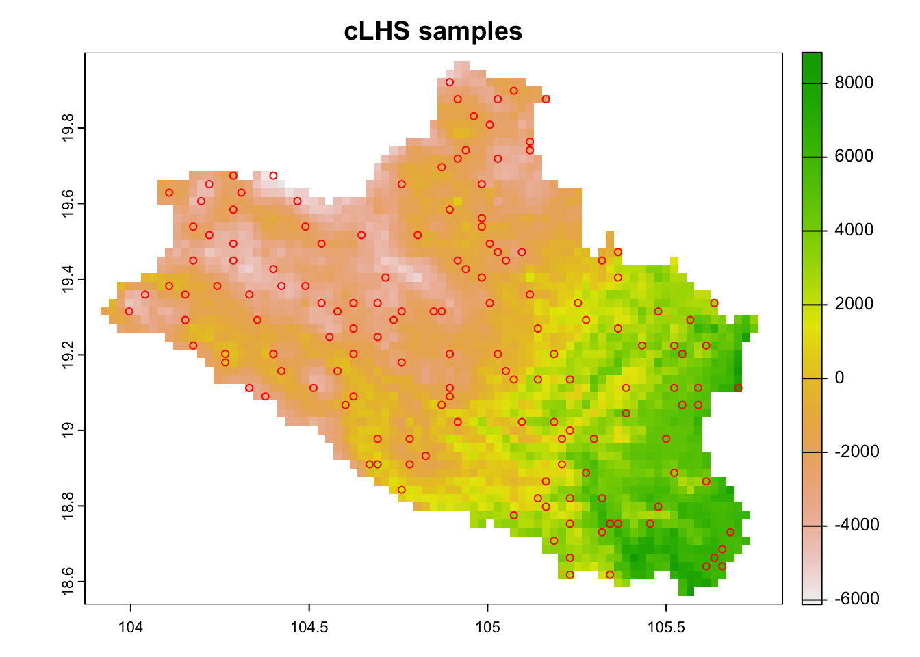
Figure 6.4: cLHS sampling points on up-scaled raster data
rm(cov.dat2)- Sampling covariate data: Other method that can be used is to sample the stack (extract the covariates information at point scale) on a regular grid at a lower resolution than the raster grid and use this information as input. The creation of a regular point grid on the raster stack is straightforward through the function
spatSamplefrom the'terra'package. In this case we create a regular grid of 1000 points.
    # Create a regular grid of 1000 points on the covariate space
    regular.sample <- spatSample(cov.dat, size = 1000, xy=TRUE, method="regular", na.rm=TRUE)
    # plot the points over the 1st raster
    plot(cov.dat[[1]], main="Regular resampled data")
    points(regular.sample, col="red", pch = 1)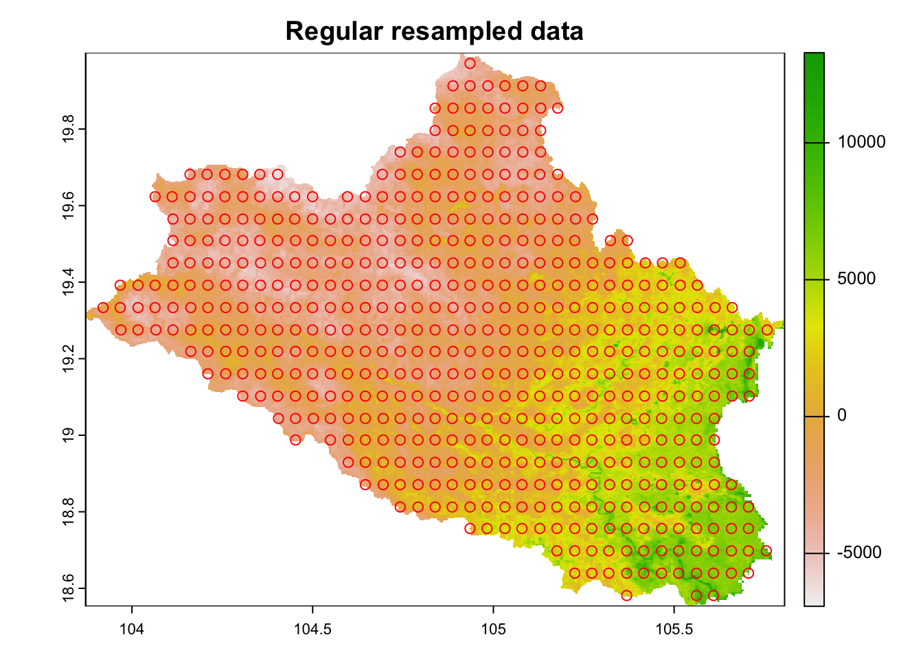
Figure 6.5: Low resolution points of covariate data
This dataframe can be directly used to get locations that best represent the covariate space in the area.
    # Create clhs samples upon the regular grid
    regular.sample.clhs <- clhs(regular.sample, size = 100, progress = FALSE, iter = 10000, simple = FALSE)
    # Plot points of clhs samples
    points <- regular.sample.clhs$sampled_data # Get point coordinates of clhs sampling
    plot(cov.dat[[1]], main="cLHS samples (red) and covariate resampled points (blue)")
    points(regular.sample, col="navy", pch = 1)
    points(points, col="red", cex=1)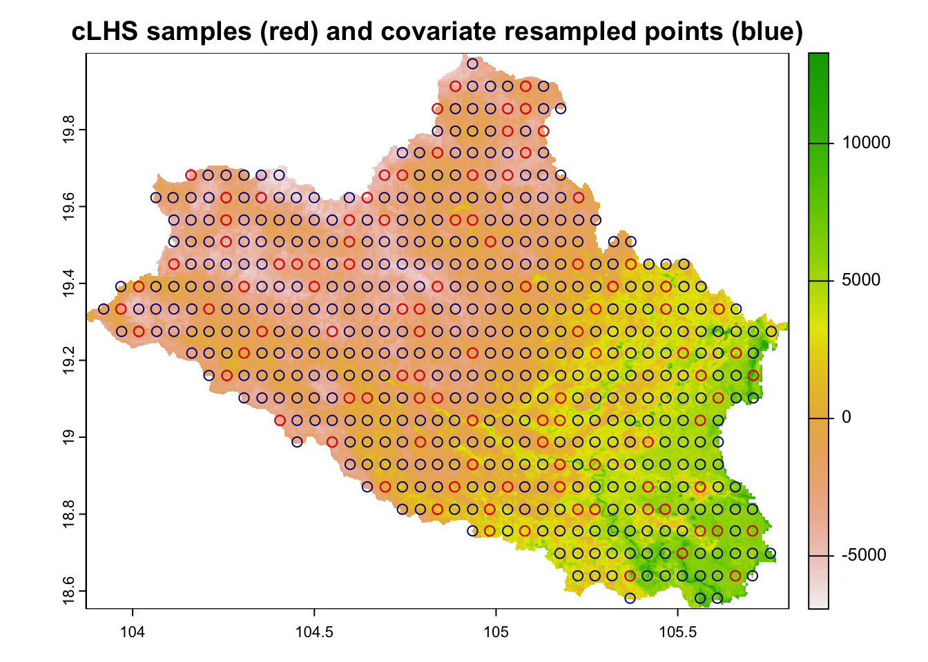
Figure 6.6: cLHS sampling points on point-grid transformed raster covariate data
Note that the sampling design follows the regular pattern of the regular grid extracted from the raster covariates
6.4 Implementation of cost–constrained cLHS sampling
There are situation in which the accessibility to some locations is totally or partially restricted such as areas with steep slopes, remote areas, or areas with forbidden access, which highly compromises the sampling process. For these cases, the sampling design can constrain the points to particular locations by defining environmental layers that cause an increment in the cost efficiency of the sampling. This is done with the cost attribute in the main 'sample_clhs' function. The following example uses the raster layer “distance to roads” as a cost layer to avoid low accessible points located at large distance from roads while optimizing the representativeness of the remaining environmental covariates.
    # Load pre-calculated distance–to–roads surface
    dist2access <- terra::rast(paste0(other.path,"nghe_d2roads.tif"))

    # Add cost surface as raster layer
    cov.dat <- c(cov.dat,dist2access)

    # Harmonize NAs
    cov.dat$dist2access <- cov.dat$dist2access * cov.dat[[1]]/cov.dat[[1]]
The sampling set is calculated using distance to roads as a cost surface.
    # Compute sampling points
    cost.clhs <- sample_clhs(cov.dat, nSamp = minimum_n, iter = 10000, progress = FALSE, cost = 'dist2access',  use.cpp = TRUE)
## Using `dist2access` as sampling constraint.Figure 6.7 shows the distribution of the cost constrained 'clhs' sampling over the 'cost' surface. The sampling procedure concentrates, as much as possible, sampling sites in locations with lower costs.
  # Plot samples
    plot(cov.dat[['dist2access']], main="cLHS samples with 'cost' constraints")
    plot(cost.clhs, col="red", cex=1,add=T)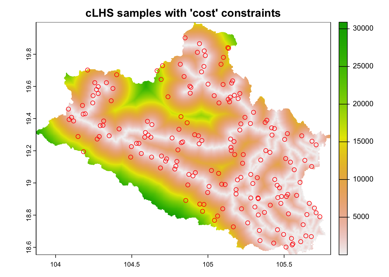
Figure 6.7: cLHS sampling with cost layers
Cost surfaces can be defined by other parameters than distances to roads. They can represent private property boundaries, slopes, presence of wetlands, etc. The package 'sgsR' implements functions to define both cost surfaces and distances to roads simultaneously. In this case, it is possible to define an inner buffer distance – i.e. the distance from the roads that should be avoided for sampling and an outer buffer – i.e. the maximum sampling distance) from roads to maximize the variability of the sampling point while considering these limits. The 'sample_clhs' function in this package also includes options to include existing legacy data in the process of clhs sampling.
    # Load legacy data
    legacy <- sf::st_read(file.path(paste0(shp.path,"/legacy_soils.shp")),quiet=TRUE)

    # Add slope to the stack
    cov.dat$slope <- slope
    # Calculate clhs points with legacy, cost and buffer to roads
    buff_inner=20;
    buff_outer=3000
    # Convert roads to sf object and cast to multilinestring
    roads <- st_as_sf(roads) %>%
      st_cast("MULTILINESTRING")

    # Calculate clhs samples using slope as cost surface, distance to roads as
    # access limitations, and including existing legacy data
    aa <- sgsR::sample_clhs(mraster = cov.dat, nSamp = minimum_n, existing = legacy,
                            iter = 10000, details = TRUE, cost="slope", access=roads,
                            buff_inner=buff_inner, buff_outer=buff_outer)
Legacy data is represented as blue dots while new samples from cLHS analyses are in red colour (Fig.6.7). Note that the new sampling points are located within a distance buffer of 20-3000 meters from roads. In addition, a cost surface has also been included in the analyses.
    ## Plot distances, roads, clhs points and legacy data
    plot(cov.dat$dist2access, main="New (red) and existing (blue) samples")
    plot(roads,add=TRUE, col="gray60")
    plot(aa$samples[aa$samples$type=="new",], col= "tomato",add=TRUE)
    plot(aa$samples[aa$samples$type=="existing",], col= "dodgerblue2",add=TRUE)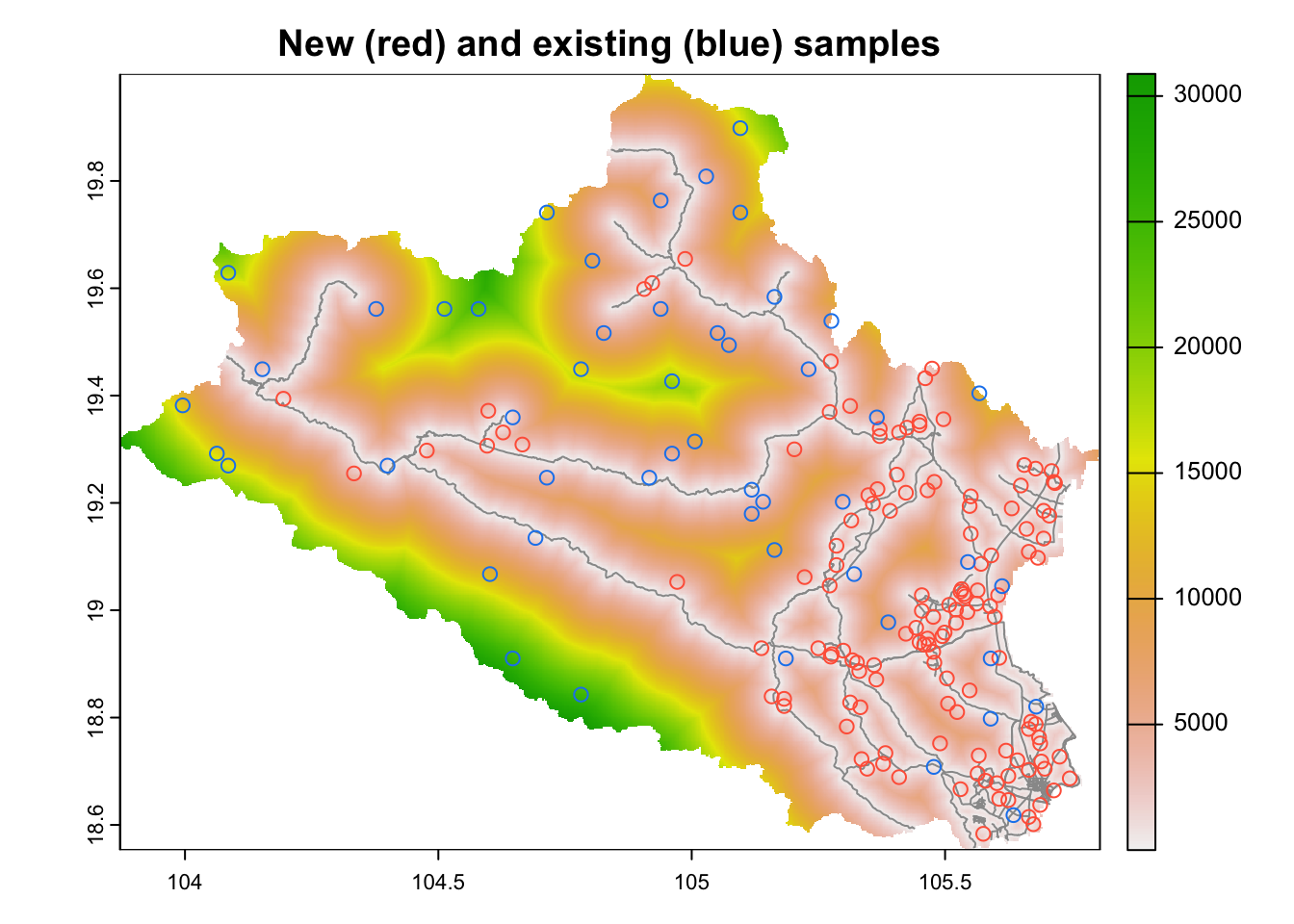
Figure 6.8: cLHS sampling with legacy data, cost surface and distance buffers around roads
The results can then be saved to a shapefile.
    # Write samples as shapefile
    aa$samples[c("type","dist2access")] %>%
      st_write(paste0(results.path,'const_clhs.shp'), delete_dsn = TRUE)
6.5 Replacement areas in cLHS design
The 'cLHS' package incorporates methods for the delineation of replacement locations that could be utilized in the case any sampling point is unreachable. In this case, the function determines the probability of similarity to each point in an area determined by a buffer distance around the points. The inputs of the 'similarity_buffer' functions must be a ‘RasterStack’ in the covariates and a ‘SpatialPointsDataFrame’ for the point data.
  ## Determine the similarity to points in a buffer of distance D
    gw <- similarity_buffer(raster::stack(cov.dat) ,  as(cost.clhs, "Spatial"), buffer = D)
The similarity probabilities for the first cLHS point is presented on Figure 6.9 over the elevation layer.
    # Plot results
    plot(elevation, legend=TRUE,main=paste("Similarity probability over elevation"))
    ## Overlay points
    points(cost.clhs, col = "dodgerblue", pch = 3)
    ## Overlay probability stack for point 1
    colors <- c((RColorBrewer::brewer.pal(9, "YlOrRd")))
    terra::plot(gw[[1]], add=TRUE ,  legend=FALSE, col=colors)
    ## Overlay 1st cLHS point
    points(cost.clhs[1,], col = "red", pch = 12,cex=1)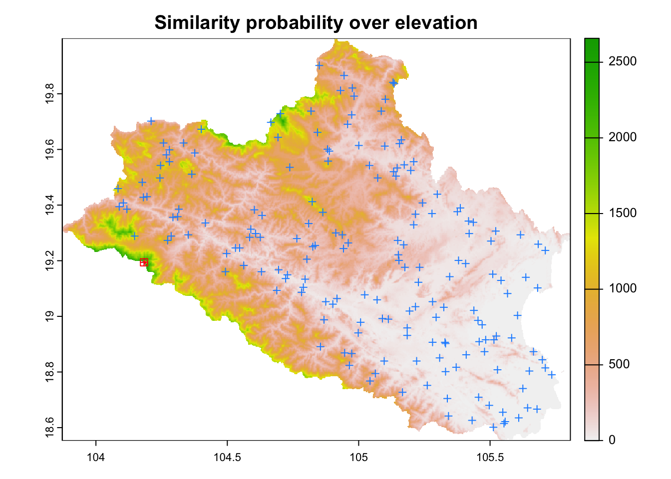
Figure 6.9: Probability of similarity in the buffer for the first cLHS point (in black) over elevation. The blue crosses represent the location of the remaining cLHS points from the analysis.
The probabilities can then be reclassified using a threshold value to delineate the areas with higher similarity to each central target point.
    # Determine a threshold break to delineate replacement areas
    similarity_threshold <- 0.90
    # Reclassify buffer raster data according to the threshold break of probability
    # 1 = similarity >= similarity_break; NA =  similarity <  similarity_break
    # Define a vector with the break intervals and the output values (NA,1)
    breaks <- c(0, similarity_threshold, NA, similarity_threshold, 1, 1)
    # Convert to a matrix
    breaks <- matrix(breaks, ncol=3, byrow=TRUE)
    # Reclassify the data in the layers from probabilities to (NA,)
    s = stack(lapply(1:raster::nlayers(gw), function(i){raster::reclassify(gw[[i]], breaks, right=FALSE)}))
The reclassified raster stack is then converted to an object of 'SpatialPolygonsDataFrame' class.
    # Polygonize replacement areas
    s = lapply(as.list(s), rasterToPolygons, dissolve=TRUE)
    s <- bind(s,keepnames=TRUE)
    # Add the identifier of the corresponding target point
    for(i in 1: length(s)){
      s@data$ID[i] <- as.integer(stringr::str_replace(s@polygons[[i]]@ID,"1.",""))
    }
    # Clean the data by storing target ID data only
    s@data <- s@data["ID"]
The results are shown in Figure 6.10.
    # Plot results
    plot(cov.dat[[1]], main=paste("cLHS samples and replacement areas for threshold = ", similarity_threshold))
    plot(s,add=TRUE, col=NA, border="gray40")
    points(cost.clhs, col="red", pch = 3)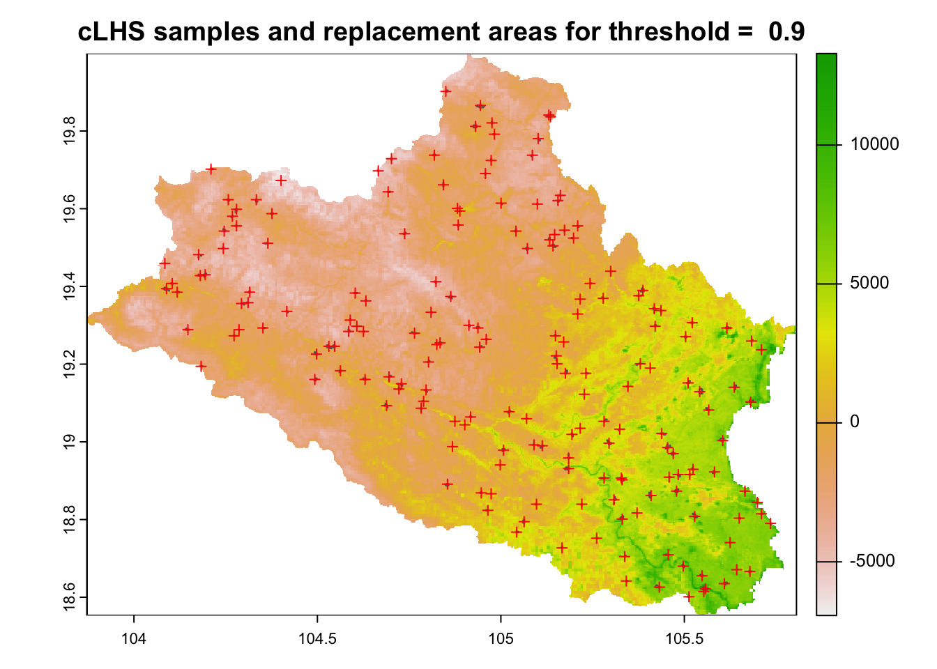
Figure 6.10: Distribution of cLHS sampling points in the study area
Replacement areas and sampling points can finally be stored as 'shapefiles'.
    # Export replacement areas to shapefile
    s <- st_as_sf(s)
    st_write(s, file.path(paste0(results.path,'replacement_areas_', D, '.shp')), delete_dsn = TRUE)

    # Write cLHS sampling points to shapefile
    cost.clhs$ID <- row(cost.clhs)[,1] # Add identifier
    out.pts <- st_as_sf(cost.clhs)
    st_write(out.pts, paste0(results.path,'target_clhs.shp'), delete_dsn = TRUE)