 Soil Sampling Design
Chapter 4 Determining the minimum sampling size
Several strategies exist for designing soil sampling, including regular, random, and stratified sampling. Each strategy comes with its own set of advantages and limitations, which must be carefully considered before commencing a soil sampling campaign. Regular sampling, also called grid sampling, is straightforward and ensures uniform coverage, making it suitable for spatial analysis and detecting trends. However, it may introduce bias and miss small–scale variability. Generally, random sampling may require a larger number of samples to accurately capture soil variability compared to stratified sampling, which is more targeted. Nonetheless, from a statistical standpoint, random sampling is often preferred. It effectively minimizes selection bias by giving every part of the study area an equal chance of being selected. This approach yields a sample that is truly representative of the entire population, leading to more accurate, broadly applicable conclusions. Random sampling also supports valid statistical inferences, ensures reliability of results, and simplifies the estimation of errors, thereby facilitating a broad spectrum of statistical analyses.
The determination of both the number and locations of soil samples is an important element in the success of any sampling campaign. The chosen strategy directly influences the representativeness and accuracy of the soil data collected, which in turn impacts the quality of the conclusions drawn from the study.
In this manual, we make use of the data from Vietnam as stored in the Google Earth repository of FAO-GPS (digital-soil-mapping-gsp-fao) for the Nghe An province. We want to determine the minimal number of soil samples that must be collated to capture at least the 95% of variability within the environmental covariates. The procedure start with random distribution of a low number of samples in the area, determine the values of the spatial covariates, and compare them with those representing the whole diversity in the area at pixel scale. The comparisons are made using the 'Kullback–Leibler divergence (KL)' – a measure of how the probability distribution of the information in the samples is different from that of the Population, i.e. the covariate space. We also calculate the '% of representativeness' as the percent of variability in the covariate information for the complete area related to the variability of covariate information in the sample dataset.
The initial section of the script is related to set–up options in the methodology. We load of R packages, define the working directory, load covariate data, and store it as SpatRaster object. Variables related to several aspects of the analyses, such as the aggregation factor of covariates (optional), the creation of a raster stack object(required in the clhs function), the initial and final number of samples in the trials, the increment step between trials, and the number of iterations within each trial, are also defined.
# Path to rasters
  raster.path <- "data/rasters"
# Path to shapes
  shp.path <- "data/shapes"
# Path to results
  results.path <- "data/results/"
# Path to additional data
  other.path <- "data/other/"
# Aggregation factor for up-scaling raster covariates (optional)
  agg.factor = 5
As in the previous section, covariates are PCA-transformed to avoid collinearity in the data and Principal Component rasters representing 99% of the information are retained for the analyses.
  ## Load raster covariate data
  # Read Spatial data covariates as rasters with terra
  cov.dat <-  list.files(raster.path, pattern = "tif$",  recursive = TRUE, full.names = TRUE)
  cov.dat <- terra::rast(cov.dat) # SpatRaster from terra
  # Aggregate stack to simplify data rasters for calculations
  cov.dat <- aggregate(cov.dat, fact=agg.factor, fun="mean")

  # Load shape of district
  nghe <- sf::st_read(file.path(paste0(shp.path,"/Nghe_An.shp")),quiet=TRUE)

  # Crop covariates on administrative boundary
  cov.dat <- crop(cov.dat, nghe, mask=TRUE)

  # Simplify raster information with PCA
  pca <- raster_pca(cov.dat)

  # Get SpatRaster layers
  cov.dat <- pca$PCA
  # Create a raster stack to be used as input in the clhs::clhs function
  cov.dat.ras <- raster::stack(cov.dat)
  # Subset rasters
  cov.dat <- pca$PCA[[1:first(which(pca$summaryPCA[3,]>0.99))]]
  cov.dat.ras <-  cov.dat.ras[[1:first(which(pca$summaryPCA[3,]>0.99))]]
  # convert to dataframe
  cov.dat.df <- as.data.frame(cov.dat)
Fig. 4.1 shows the covariates retained for the analyses.
  ## Plot covariates
   plot(cov.dat)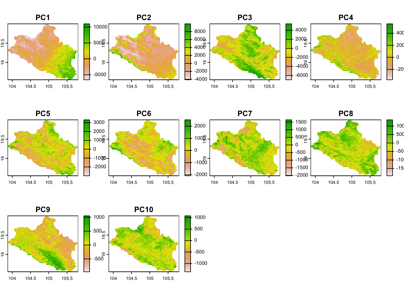
Figure 4.1: Plot of the covariates
  ## Define the number of samples to be tested in a loop (from initial to final) and the step of the sequence
  initial.n <- 50 # Initial sampling size to test
  final.n <- 300 # Final sampling size to test
  by.n <- 10 # Increment size
  iters <- 10 # Number of trials on each size
The second section is where the analyses of divergence and representativeness of the sampling scheme are calculated.
The analyses are performed in a loop using growing numbers of samples at each trial. Some empty vectors are defined to store the output results at each loop. At each trial of sample size 'N', soil samples are located at locations where the amount of information in the covariates is maximized according to the conditioned Latin Hypercube sampling method in the 'clhs' package (Roudier et al., 2011). A number of 10 replicates are calculated to determine the amount inter–variability in KL divergence and representativeness in the trial. The final results for each sample size correspond to the mean results obtained from each iteration at the corresponding sample size. The minimum sample size selected correspond to the size that accounts for at least 95% of the variability of information in the covariates within the area. The optimal sampling schema proposed correspond to the random scheme at the minimum sample size with higher value of representativeness.
  # Define empty vectors to store results
  number_of_samples <- c()
  prop_explained <- c()
  klo_samples <-c()
  samples_storage <- list()

  for (trial in seq(initial.n, final.n, by = by.n)) {
    for (iteration in 1:iters) {
      # Generate stratified clhs samples
      p.dat_I <-  clhs(cov.dat.ras,
          size = trial, iter = 10000,
          progress = FALSE, simple = FALSE)

      # Get covariate values for each point
      p.dat_I <- p.dat_I$sampled_data
      # Get the covariate values at points as dataframe and delete NAs
      p.dat_I.df <- as.data.frame(p.dat_I@data) %>%
        na.omit()

      # Store samples as list with point coordinates
      samples_storage[[paste0("N", trial, "_", iteration)]] <- p.dat_I

      ## Comparison of population and sample distributions - Kullback-Leibler (KL) divergence
      # Define quantiles of the study area (number of bins)
      nb <- 25
      # Quantile matrix of the covariate data
      q.mat <- matrix(NA, nrow = (nb + 1), ncol = nlyr(cov.dat))
      j = 1
      for (i in 1:nlyr(cov.dat)) {
        ran1 <- minmax(cov.dat[[i]])[2] - minmax(cov.dat[[i]])[1]
        step1 <- ran1 / nb
        q.mat[, j] <-
          seq(minmax(cov.dat[[i]])[1],
              to = minmax(cov.dat[[i]])[2],
              by = step1)
        j <- j + 1
      }
      # q.mat

      # Hypercube of covariates in study area
      # Initialize the covariate matrix
      cov.mat <- matrix(1, nrow = nb, ncol = ncol(q.mat))
      cov.dat.mx <- as.matrix(cov.dat.df)
      for (i in 1:nrow(cov.dat.mx)) {
        for (j in 1:ncol(cov.dat.mx)) {
          dd <- cov.dat.mx[[i, j]]

          if (!is.na(dd)) {
            for (k in 1:nb) {
              kl <- q.mat[k, j]
              ku <- q.mat[k + 1, j]

              if (dd >= kl && dd <= ku) {
                cov.mat[k, j] <- cov.mat[k, j] + 1
              }
            }
          }
        }
      }

      # Compare whole study area covariate space with the selected sample
      # Sample data hypercube (the same as for the raster data but on the sample data)
      h.mat <- matrix(1, nrow = nb, ncol = ncol(q.mat))
      for (i in 1:nrow(p.dat_I.df)) {
        for (j in 1:ncol(p.dat_I.df)) {
          dd <- p.dat_I.df[i, j]

          if (!is.na(dd)) {
            for (k in 1:nb) {
              kl <- q.mat[k, j]
              ku <- q.mat[k + 1, j]

              if (dd >= kl && dd <= ku) {
                h.mat[k, j] <- h.mat[k, j] + 1
              }
            }
          }
        }
      }

      ## Compute Kullback-Leibler (KL) divergence
      kl.index <- c()
      for (i in 1:ncol(cov.dat.df)) {
        kl <-    KL.empirical(c(cov.mat[, i]), c(h.mat[, i]))
        kl.index <- c(kl.index, kl)
        klo <-  mean(kl.index)
      }

      ## Calculate the proportion of "env. variables" in the covariate spectra that fall within the convex hull of variables in the "environmental sample space"
      # Principal component of the data sample
      pca.s = prcomp(p.dat_I.df, scale = TRUE, center = TRUE)
      scores_pca1 = as.data.frame(pca.s$x)
      # Plot the first 2 principal components and convex hull
      rand.tr <-
        tri.mesh(scores_pca1[, 1], scores_pca1[, 2], "remove") # Delaunay triangulation
      rand.ch <- convex.hull(rand.tr, plot.it = F) # convex hull
      pr_poly <-
        cbind(x = c(rand.ch$x), y = c(rand.ch$y)) # save the convex hull vertices
      # PCA projection of study area population onto the principal components
      PCA_projection <-
        predict(pca.s, cov.dat.df) # Project study area population onto sample PC
      newScores = cbind(x = PCA_projection[, 1], y = PCA_projection[, 2]) # PC scores of projected population
      # Check which points fall within the polygon
      pip <-
        point.in.polygon(newScores[, 2], newScores[, 1], pr_poly[, 2], pr_poly[, 1], mode.checked =
                           FALSE)
      newScores <- data.frame(cbind(newScores, pip))
      klo_samples <- c(klo_samples, klo)
      prop_explained <-
        c(prop_explained, sum(newScores$pip) / nrow(newScores) * 100)
      number_of_samples <- c(number_of_samples, trial)
      # print(
      #   paste(
      #     "N samples = ",
      #     trial,
      #     " out of ",
      #     final.n,
      #     "; iteration = ",
      #     iteration,
      #     "; KL = ",
      #     klo,
      #     "; Proportion = ",
      #     sum(newScores$pip) / nrow(newScores) * 100
      #   )
      # )
    }
  }
Figure 4.2 shows the distribution of covariates in the sample space, and Figure 4.3 indicates the variability in the estimations of KL divergence and repressentativeness percent in the 10 within each sample size.
  # Plot the polygon and all points to be checked
     plot(newScores[,1:2], xlab="PCA 1", ylab="PCA 2",
          xlim=c(min(newScores[,1:2], na.rm = T), max(newScores[,1:2], na.rm = T)),
          ylim=c(min(newScores[,1:2], na.rm = T), max(newScores[,1:2], na.rm = T)),
          col='black',
          main='Environmental space plots over the convex hull of soil legacy data')

     polygon(pr_poly,col='#99999990')

  # # Plot points outside convex hull
     points(newScores[which(newScores$pip==0),1:2], col='red', pch=12, cex =1)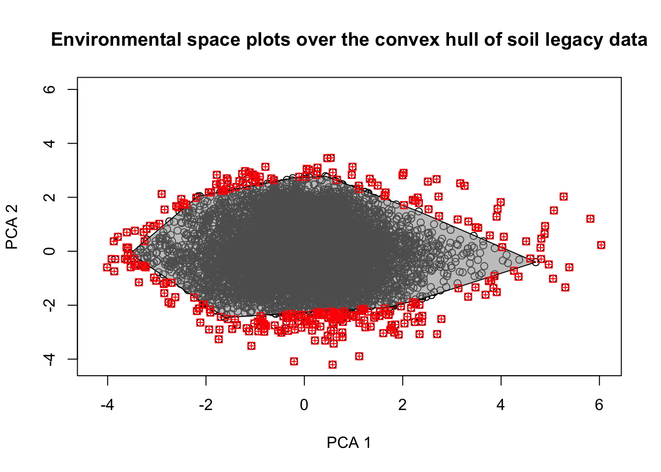
Figure 4.2: Distribution of covariates in the sample space
  ## Plot dispersion on KL and % by N
  par(mar = c(5, 4, 5, 5))
  boxplot(Perc ~ N, data=results, col = rgb(1, 0.1, 0, alpha = 0.5),ylab = "%")
  mtext("KL divergence",side=4,line=3)
  # Add new plot
  par(new = TRUE,mar=c(5, 4, 5, 5))
  # Box plot
  boxplot(KL ~ N, data=results, axes = FALSE,outline = FALSE,
          col = rgb(0, 0.8, 1, alpha = 0.5), ylab = "")
  axis(4, at=seq(0.02, 0.36, by=.06),  label=seq(0.02, 0.36, by=.06), las=3)
  # Draw legend
  par(xpd=TRUE)
  legend("top", inset=c(1,-.15) ,c("% coincidence", "KL divergence"), horiz=T,cex=.9,
         box.lty=0,fill = c(rgb(1, 0.1, 0, alpha = 0.5), rgb(0, 0.8, 1, alpha = 0.5)))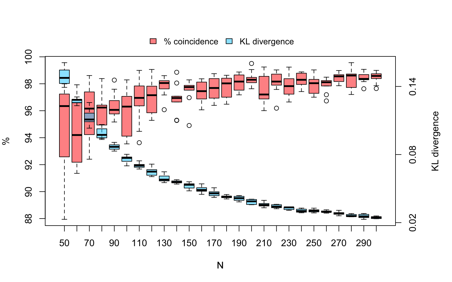
Figure 4.3: Boxplot of the dispersion in KL and % repressentativeness in the iteration trials for each sample size
We determine the minimum sample size and plot the evaluation results.
The following figure shows the cumulative distribution function (cdf) of the KL divergence and the % of representativeness with growing sample sizes. Representativeness increases with the increasing sample size, while KL divergence decreases as expected. The red dot identifies the trial with the minimum sample size for the area in relation to the covariates analysed.
  ## Plot cdf and minimum sampling point
  x <- xx
  y <- normalized

  mydata <- data.frame(x,y)
  opti <- mydata[mydata$x==minimum_n,]

  plot_ly(mydata,
          x = ~x,
          y = ~normalized,
          mode = "lines+markers",
          type = "scatter",
          name = "CDF (1–KL divergence)") %>%
    add_trace(x = ~x,
              y = ~jj,
              mode = "lines+markers",
              type = "scatter",
              yaxis = "y2",
              name = "KL divergence")  %>%
    add_trace(x = ~opti$x,
              y = ~opti$y,
              yaxis = "y",
              mode = "markers",
              name = "Minimum N",
              marker = list(size = 8, color = '#d62728',line = list(color = 'black', width = 1))) %>%
    layout(xaxis = list(title = "N",
                        showgrid = T,
                        dtick = 50,
                        tickfont = list(size = 11)),
           yaxis = list(title = "1–KL divergence (% CDF)", showgrid = F ),
           yaxis2 = list(title = "KL divergence",
                         overlaying = "y", side = "right"),
           legend = list(orientation = "h", y = 1.2, x = 0.1,
                         traceorder = "normal"),
           margin = list(t = 50, b = 50, r = 100, l = 80),
           hovermode = 'x')  %>%
    config(displayModeBar = FALSE)
Figure 4.4: KL Divergence and Proportion of Representativeness as function of sample size
According to Figure 4.4, the minimum sampling size for the area, which captures at least 95% of the environmental variability of covariates is N = 182.
Finally, we can determine the optimal distribution of samples over the study area according to these specific results, taking into account the minimum sampling size and the increasing interval in the sample size. The results are shown in Figure 4.5.
## Determine the optimal iteration according to the minimum N size
  optimal_iteration <- results[which(abs(results$N - minimum_n) == min(abs(results$N - minimum_n))),] %>%
    mutate(IDX = 1:n()) %>%
    filter(Perc==max(Perc))

  # Plot best iteration points
  N_final <- samples_storage[paste0("N",optimal_iteration$N,"_", optimal_iteration$IDX)][[1]]
  plot(cov.dat[[1]])
  points(N_final)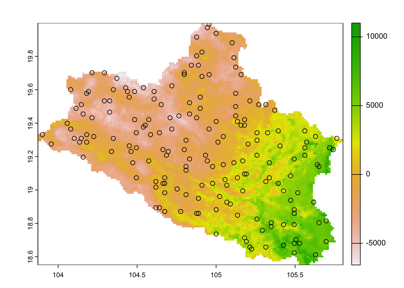
Figure 4.5: Covariates and optimal distribution of samples
In summary, we utilize the variability within the covariate data to ascertain the minimum number of samples required to capture a minimum of 95% of this variability. Our approach involves assessing the similarities in variability between the sample space and the population space (study area) through calculations of the Kullback–Leibler (KL) divergence and the percentage of similarity at various stages of increasing sample sizes. These results are then utilized to fit a model representing the expected distribution of representativeness as a function of sample size. This model guides us in determining the minimum sample size necessary to achieve a representation of at least 95% of the environmental diversity within the area