 Global Soil Nutrient and Nutrient Budgets maps (GSNmap) Phase I
Chapter 7 Step 2: download environmental covariates
7.1 Environmental covariates
The SCORPAN equation (Eq. (4.1)) refers to the soil-forming factors that determine the spatial variation of soils. However, these factors cannot be measured directly. Instead, proxies of these soil forming factors are used. One essential characteristic of the environmental covariates is that they are spatially explicit, covering the whole study area. The following Table ?? lists all the environmental covariates that can be implemented under the present DSM framework. Apart from the environmental covariates mentioned in Table ??, other types of maps could also be included, such as Global Surface Water Mapping Layers and Water Soil Erosion from the Joint Research Centre (JRC). At national level there may be very significant covariates that could complement or replace the covariates of Table ??. Thus, the selection of suitable covariate layers needs to be assessed with common sense and applying expert knowledge.
7.2 Download covariates and cropland mask with Google Earth Engine (GEE)
The following are the steps to access and download the environmental covariates and cropland mask. The GSP has streamlined the process of downloading environmental covariates clipped to national borders from GEE. This chapter aims to guide you on how to download environmental covariates using a GEE script written in JavaScript.
You can find the JavaScript code in the material provided in this technical manual under 03-scripts/3.0.Download_Covariates_&_Mask.txt. To use the code, simply copy and paste the text in the GEE console as shown in the figure below.
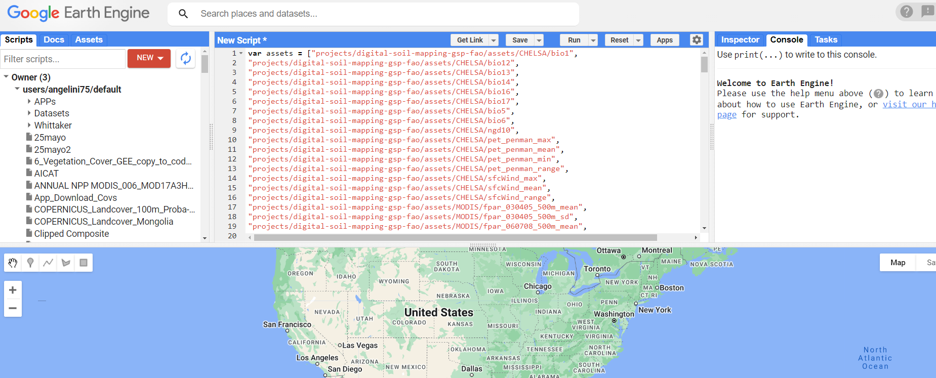
Figure 7.1: Copy and paste script in the code editor.
If not done already, it is necessary to specify the working directory and a file path directory to the output folder where the clipped covariate layers are going to be saved. In case users want to use their own shapefile of the AOI, it is necessary to specify the file path to load it into our R session later. Alternatively, the shapefile of the AOI can be clipped from the official UN map shapefile that is available in the “Digital-Soil-Mapping-GSP-FAO” based on the 3-digit ISO code (ISO3CD column in the attribute table). The process to do this will be explained in a few steps. Finally, it is also necessary to specify the resolution to 250 x 250 m for the covariate layers and set the CRS to WGS84 (equals EPSG code 4326). Note that the target resolution of the GSNmap is at 250 m, which can be considered a moderate resolution for a global layer. However, those countries that require a higher resolution are free to develop higher resolution maps and aggregate the resulting maps to the target resolution of GSNmap for submission.
The following text explains the structure of the script that will be executed in GEE, and which parts of the script need to be modified to extract the covariates from the area of interest (AOI).
7.2.1 Assets
In GEE, an “asset” refers to any data or code that has been uploaded and stored in GEE’s cloud-based servers. Assets can include remote sensing data, vector data, and even scripts or functions.
The following code reads the assets that have been created by the GSP in GEE. This means that the code accesses the data and scripts that GSP has uploaded to GEE, and uses them to perform specific tasks or analyses. By leveraging GEE’s cloud-based infrastructure and GSP’s assets, users can easily access and analyze large amounts of data without the need for local storage or processing power.
#Empty environment and cache
var assets =
["projects/digital-soil-mapping-gsp-fao/assets/CHELSA/bio1",
"projects/digital-soil-mapping-gsp-fao/assets/CHELSA/bio12",
"projects/digital-soil-mapping-gsp-fao/assets/CHELSA/bio13",
"projects/digital-soil-mapping-gsp-fao/assets/CHELSA/bio14",
"projects/digital-soil-mapping-gsp-fao/assets/CHELSA/bio16",
"projects/digital-soil-mapping-gsp-fao/assets/CHELSA/bio17",
"projects/digital-soil-mapping-gsp-fao/assets/CHELSA/bio5",
"projects/digital-soil-mapping-gsp-fao/assets/CHELSA/bio6",
"projects/digital-soil-mapping-gsp-fao/assets/CHELSA/ngd10",
"projects/digital-soil-mapping-gsp-fao/assets/CHELSA/pet_penman_max",
"projects/digital-soil-mapping-gsp-fao/assets/CHELSA/pet_penman_mean",
"projects/digital-soil-mapping-gsp-fao/assets/CHELSA/pet_penman_min",
"projects/digital-soil-mapping-gsp-fao/assets/CHELSA/pet_penman_range",
"projects/digital-soil-mapping-gsp-fao/assets/CHELSA/sfcWind_max",
"projects/digital-soil-mapping-gsp-fao/assets/CHELSA/sfcWind_mean",
"projects/digital-soil-mapping-gsp-fao/assets/CHELSA/sfcWind_range",
"projects/digital-soil-mapping-gsp-fao/assets/MODIS/fpar_030405_500m_mean",
"projects/digital-soil-mapping-gsp-fao/assets/MODIS/fpar_030405_500m_sd",
"projects/digital-soil-mapping-gsp-fao/assets/MODIS/fpar_060708_500m_mean",
"projects/digital-soil-mapping-gsp-fao/assets/MODIS/fpar_060708_500m_sd",
"projects/digital-soil-mapping-gsp-fao/assets/MODIS/fpar_091011_500m_mean",
"projects/digital-soil-mapping-gsp-fao/assets/MODIS/fpar_091011_500m_sd",
"projects/digital-soil-mapping-gsp-fao/assets/MODIS/fpar_120102_500m_mean",
"projects/digital-soil-mapping-gsp-fao/assets/MODIS/fpar_120102_500m_sd",
"projects/digital-soil-mapping-gsp-fao/assets/MODIS/lstd_030405_mean",
"projects/digital-soil-mapping-gsp-fao/assets/MODIS/lstd_030405_sd",
"projects/digital-soil-mapping-gsp-fao/assets/MODIS/lstd_060708_mean",
"projects/digital-soil-mapping-gsp-fao/assets/MODIS/lstd_060708_sd",
"projects/digital-soil-mapping-gsp-fao/assets/MODIS/lstd_091011_mean",
"projects/digital-soil-mapping-gsp-fao/assets/MODIS/lstd_091011_sd",
"projects/digital-soil-mapping-gsp-fao/assets/MODIS/lstd_120102_mean",
"projects/digital-soil-mapping-gsp-fao/assets/MODIS/lstd_120102_sd",
"projects/digital-soil-mapping-gsp-fao/assets/MODIS/ndlst_030405_mean",
"projects/digital-soil-mapping-gsp-fao/assets/MODIS/ndlst_030405_sd",
"projects/digital-soil-mapping-gsp-fao/assets/MODIS/ndlst_060708_mean",
"projects/digital-soil-mapping-gsp-fao/assets/MODIS/ndlst_060708_sd",
"projects/digital-soil-mapping-gsp-fao/assets/MODIS/ndlst_091011_mean",
"projects/digital-soil-mapping-gsp-fao/assets/MODIS/ndlst_091011_sd",
"projects/digital-soil-mapping-gsp-fao/assets/MODIS/ndlst_120102_mean",
"projects/digital-soil-mapping-gsp-fao/assets/MODIS/ndlst_120102_sd",
"projects/digital-soil-mapping-gsp-fao/assets/MODIS/ndvi_030405_250m_mean",
"projects/digital-soil-mapping-gsp-fao/assets/MODIS/ndvi_030405_250m_sd",
"projects/digital-soil-mapping-gsp-fao/assets/MODIS/ndvi_060708_250m_mean",
"projects/digital-soil-mapping-gsp-fao/assets/MODIS/ndvi_060708_250m_sd",
"projects/digital-soil-mapping-gsp-fao/assets/MODIS/ndvi_091011_250m_mean",
"projects/digital-soil-mapping-gsp-fao/assets/MODIS/ndvi_091011_250m_sd",
"projects/digital-soil-mapping-gsp-fao/assets/MODIS/ndvi_120102_250m_mean",
"projects/digital-soil-mapping-gsp-fao/assets/MODIS/ndvi_120102_250m_sd",
"projects/digital-soil-mapping-gsp-fao/assets/MODIS/snow_cover",
"projects/digital-soil-mapping-gsp-fao/assets/MODIS/swir_060708_500m_mean",
"projects/digital-soil-mapping-gsp-fao/assets/LANDCOVER/crops",
"projects/digital-soil-mapping-gsp-fao/assets/LANDCOVER/flooded_vegetation",
"projects/digital-soil-mapping-gsp-fao/assets/LANDCOVER/grass",
"projects/digital-soil-mapping-gsp-fao/assets/LANDCOVER/shrub_and_scrub",
"projects/digital-soil-mapping-gsp-fao/assets/LANDCOVER/trees",
"projects/digital-soil-mapping-gsp-fao/assets/OPENLANDMAP/dtm_curvature_250m",
"projects/digital-soil-mapping-gsp-fao/assets/OPENLANDMAP/dtm_downslopecurvature_250m",
"projects/digital-soil-mapping-gsp-fao/assets/OPENLANDMAP/dtm_dvm2_250m",
"projects/digital-soil-mapping-gsp-fao/assets/OPENLANDMAP/dtm_dvm_250m",
"projects/digital-soil-mapping-gsp-fao/assets/OPENLANDMAP/dtm_elevation_250m",
"projects/digital-soil-mapping-gsp-fao/assets/OPENLANDMAP/dtm_mrn_250m",
"projects/digital-soil-mapping-gsp-fao/assets/OPENLANDMAP/dtm_neg_openness_250m",
"projects/digital-soil-mapping-gsp-fao/assets/OPENLANDMAP/dtm_pos_openness_250m",
"projects/digital-soil-mapping-gsp-fao/assets/OPENLANDMAP/dtm_slope_250m",
"projects/digital-soil-mapping-gsp-fao/assets/OPENLANDMAP/dtm_tpi_250m",
"projects/digital-soil-mapping-gsp-fao/assets/OPENLANDMAP/dtm_twi_500m",
"projects/digital-soil-mapping-gsp-fao/assets/OPENLANDMAP/dtm_upslopecurvature_250m",
"projects/digital-soil-mapping-gsp-fao/assets/OPENLANDMAP/dtm_vbf_250m",
"projects/digital-soil-mapping-gsp-fao/assets/POP/hfp2013_merisINT",
"projects/digital-soil-mapping-gsp-fao/assets/POP/night_lights_stable_2013",
"projects/digital-soil-mapping-gsp-fao/assets/POP/population_density_2020"];
7.2.2 Define the region of interest (ROI)
This script in GEE loads borders of a specific country or a user-defined shapefile into the workspace. It does this by creating a region of interest (ROI) based on the country borders. The script first specifies a list of countries to be included in the ROI and then loads the corresponding geometries from the ‘USDOS/LSIB_SIMPLE/2017’ feature collection in the case of the LSIB 2017 dataset. In the case of a user-defined shapefile, the script uploads the borders of the ROI as an asset and replaces ‘your_shapefile’ with the path to the uploaded shapefile. Finally, the region variable is assigned the geometry of the ROI, which can be used to clip and process data within the specified boundary. You must change either the name of the country or the shape file (as an asset) to download the covariates for your specific ROI.
// Load borders

/// Using UN 2020 (replace the countries to download)
var ISO = ['ITA'];
var aoi =
ee.FeatureCollection(
'projects/digital-soil-mapping-gsp-fao/assets/UN_BORDERS/BNDA_CTY'
)
  .filter(ee.Filter.inList('ISO3CD', ISO));
var region = aoi.geometry();

/// Using a shapefile
/// 1. Upload the borders of your countries as an asset
/// 2. Replace 'your_shapefile' with the path to your shapefile
// var shapefile =
// ee.FeatureCollection('users/your_username/your_shapefile');
// var region = shapefile.geometry();
7.2.3 Load and clip the covariates
This script loads an asset collection into an Earth Engine (EE) image collection and clips each image in the collection to a specific region of interest (ROI).
First, the ee.ImageCollection function is used to load the assets into an EE image collection. The assets variable is expected to be a list of asset IDs.
Next, the map function is applied to the image collection to clip each image to the specified ROI. The clip function clips the image to the given ROI, and toFloat() converts the data type of the clipped image to floating-point values. The result of this operation is a new EE image collection called clippedCollection, where each image has been clipped to the specified ROI.
// Load assets as ImageCollection
var assetsCollection = ee.ImageCollection(assets);

// Clip each image in the collection to the region of interest
var clippedCollection = assetsCollection.map(function(img){
  return img.clip(region).toFloat();
});
7.2.4 Clean holes in FPAR layers
The Fraction of Photosynthetically Active Radiation (FPAR) MODIS product represents the fraction of incident photosynthetically active radiation (PAR) that is absorbed by vegetation. This product is calculated from satellite-based observations of surface reflectance, and it is commonly used to estimate vegetation growth and productivity.
In some areas, the FPAR MODIS product contains no data values in areas where the vegatation is scarce or absent. To avoin transferring these holes to the digital soil maps, we covert no data values to zeroes. The rest of the script in this section is to reclip the rasters, stack them in a single object and rename them.
// Function to replace masked values with zeroes for fpar bands
function replaceMaskedFpar(img) {
  var allBands = img.bandNames();
  var fparBands =
  allBands.filter(ee.Filter.stringStartsWith('item', 'fpar'));
  var nonFparBands = allBands.removeAll(fparBands);

  var fparImg = img.select(fparBands).unmask(0);
  var nonFparImg = img.select(nonFparBands);

  // If there are no fpar bands, return the original image
  var result = ee.Algorithms.If(fparBands.length().eq(0),
                                 img,
                                 nonFparImg.addBands(fparImg));

  return ee.Image(result);
}

// Clip each image in the collection to the region
//of interest and replace masked values for fpar bands
var clippedCollection = assetsCollection.map(function(img){
  var clippedImg = img.clip(region).toFloat();
  return replaceMaskedFpar(clippedImg);
});

// Stack the layers and maintain the layer names in the final file
var stacked = clippedCollection.toBands();

// Get the list of asset names
var assetNames = ee.List(assets).map(function(asset) {
  return ee.String(asset).split('/').get(-1);
});

// Rename the bands with asset names
var renamed = stacked.rename(assetNames);
print(renamed, 'Covariates to be exported')
7.2.5 Visualize and export the covariates
This script has two main parts: visualizing the result and exporting the stacked image to Google Drive.
In the first part, the script sets a visualization parameter (visParams) to define the visualization properties of the stacked image. Specifically, the script specifies that the visualization should use the ‘bio1’ band and a color palette with four colors to represent the range of values in the band. The min and max values are also set to control the range of values that are displayed.
Next, the script adds the renamed image (renamed) to the map and applies the visualization parameters defined in visParams. The Map.centerObject() function centers the map on the renamed image, and the Map.addLayer() function adds the image layer to the map with the specified name (‘Covariates’).
In the second part of the script, the Export.image.toDrive() function is used to export the stacked image to Google Drive. This function exports the renamed image as a GeoTIFF file with the description ‘covariates’, which is saved in the ‘GEE’ folder in the user’s Google Drive (you have to either create the folder in GDrive, or indicate a different target folder). The scale parameter specifies the spatial resolution of the exported image, while the maxPixels parameter sets the maximum number of pixels that can be exported. Finally, the region parameter specifies the geographic extent of the exported image, which is set to the region variable defined earlier in the script.
// Visualize the result
// Set a visualization parameter
// (you can adjust the colors as desired)
var visParams = {
  bands: 'bio1',
  min: 19248,
  max: 46139,
  palette: ['blue', 'green', 'yellow', 'red']
};

// Add the layer to the map
Map.centerObject(renamed, 6)
Map.addLayer(renamed, visParams, 'Covariates');


// Export the stacked image to Google Drive
Export.image.toDrive({
  image: renamed,
  description: 'covariates',
  folder: 'GEE',
  scale: 250,
  maxPixels: 1e13,
  region: region
});
7.2.6 Load and clip the Copernicus land cover map and
This script loads an image collection of global land cover, selects the ‘discrete_classification’ band, and clips the image to a specified region. It then sets the CRS and spatial resolution of the output image, and applies resampling to change the spatial resolution to the desired value. The resulting image is stored in the variable image1.
/* Create mask for croplands ----------------------------*/

// Load the Copernicus Global Land Service image collection
var imageCollection =
ee.Image("COPERNICUS/Landcover/100m/Proba-V-C3/Global/2019")
  .select("discrete_classification")
  .clip(region)

var crs = 'EPSG:4326'; // WGS84
var res = 250; // Resolution in decimal degrees

// Default resampling is nearest neighbor
var image1 = imageCollection.resample()
  .reproject({
    crs: crs, // Add your desired CRS here
    scale: res // Add your desired scale here
  });
7.2.7 Reclassify the land cover map
This script reclassifies the land cover classes of the image1 using the remap function, which replaces the values in inList with the corresponding values in outList. We only keep class 40 which refer to Cultivated and managed vegetation / agriculture. The resulting image is then converted to a double data type, clipped to a specified region, and stored in the variable FAO_lu. The script then converts all 0 values in FAO_lu to NA values using the updateMask function and stores the resulting masked image in FAO_lu. The intermediate results are printed using the print function.
// Reclassify the land cover classes
var inList = [0, 20, 30, 40, 50, 60, 70, 80, 90, 100, 111,
               112, 113, 114, 115, 116,
              121, 122, 123, 124, 125, 126, 200];
var outList = [0, 0, 0, 1, 0, 0, 0, 0, 0, 0, 0, 0,
0, 0, 0, 0, 0, 0, 0, 0, 0, 0, 0];

var FAO_lu = image1.remap(inList, outList)
  .toDouble()
  .clip(region);

// print(FAO_lu)

// Convert 0 to NA
var mask = FAO_lu.neq(0);
print(mask)
FAO_lu = FAO_lu.updateMask(mask);

print(FAO_lu, "Mask")
7.2.8 Visualization and exporting mask
The code sets up visualization parameters for the reclassified land cover image and adds it as a layer to the map using the Map.addLayer function. The resulting image is then exported as a raster to Google Drive using the Export.image.toDrive function with specified parameters such as the folder to save the image, the desired scale and CRS, the region of interest, and the maximum number of pixels for export if needed. The resulting image is a binary mask where 1 represents the forest class and 0 represents all other classes.
var visParams = {
  bands: 'remapped',
  min: 0,
  max: 1,
  palette: ['green', 'yellow']
};

// Add the layer to the map
Map.addLayer(FAO_lu,visParams ,'Mask');

// Export the land cover image as a raster to Google Drive
Export.image.toDrive({
  image: FAO_lu,
  folder: 'GEE',
  description: 'mask',
  scale: res, // Add your desired scale here
  region: region,
  crs: crs, // Add your desired CRS here
  maxPixels: 1e13 // Add a maximum number of pixels for export
});
7.3 Run and export in GEE
To execute a script in GEE, you can run it by clicking the “Run” button in the upper right-hand corner of the code editor. The “Run” button in GEE executes the script and any tasks specified in the script, such as exporting files to Google Drive. The status of the task can be monitored in the “Tasks” tab.
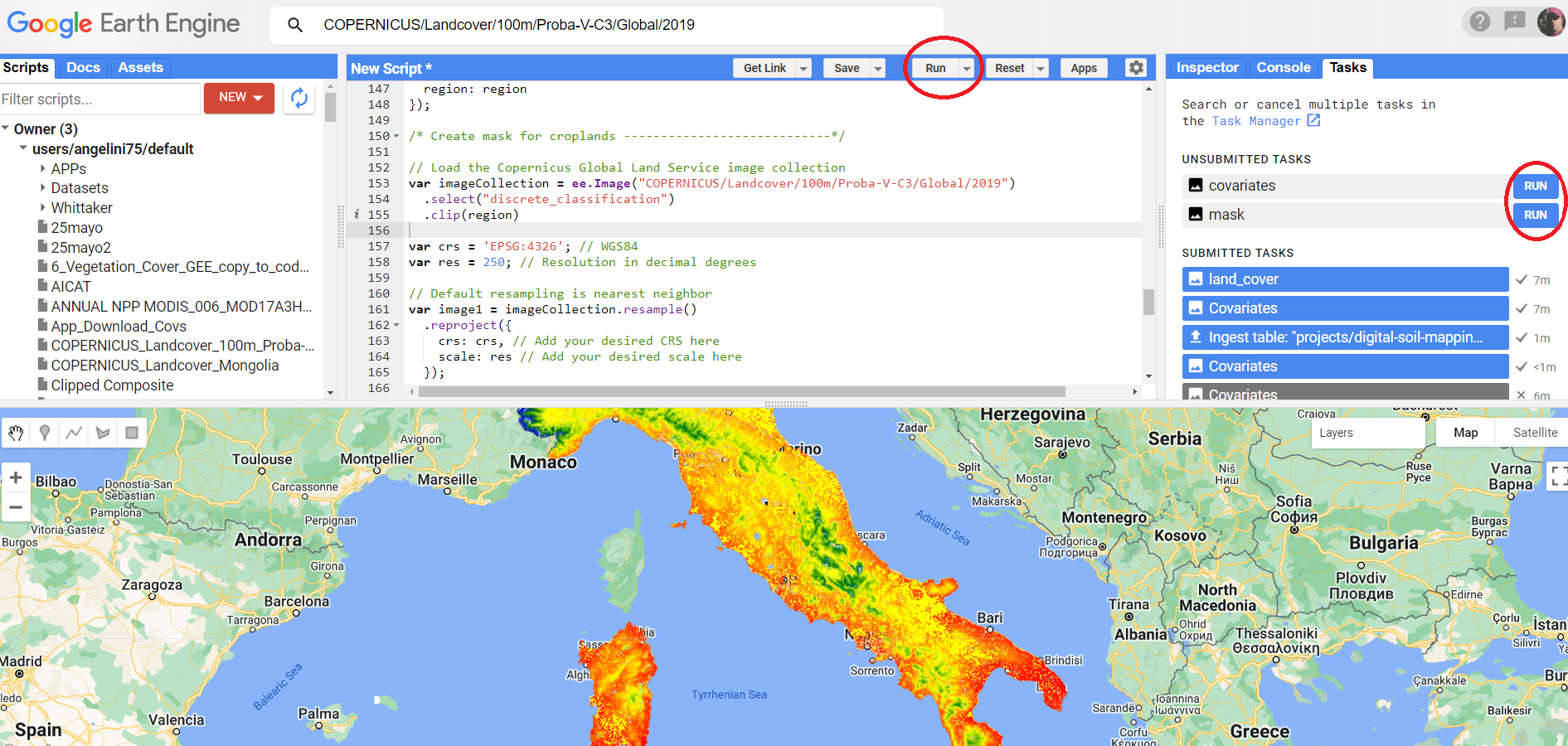
Figure 7.2: Run button in code editor and RUN task in Tasks bar.
To run a task for exporting files to Google Drive in GEE, the Export.image.toDrive() function exports the image Google Drive. To start the task, you need to RUN the task, and it will be added to the GEE task list. You can monitor its progress and download the exported file once the task is complete.