Annex III: Mapping without point coordinates

This chapter provides step-by-step instructions in case the soil measurements do not have point coordinates but come with information on the sampling region, i.e. location within an administrative unit. In this approach, soil samples are randomly distributed across the respective area (see Figure 10.1).

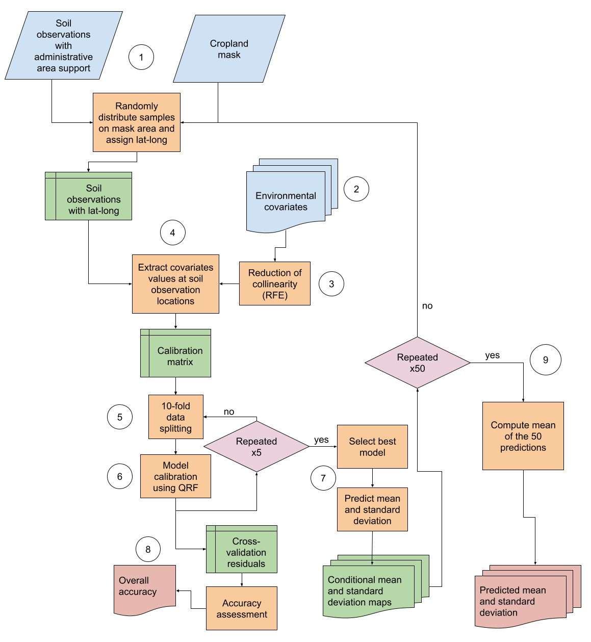
Figure 10.1: Digital soil mapping approach for area-support data. Circles are the steps.

The steps are similar to the ones specified in Step 3. After merging the soil and environmental covariate data, the ones with most explanatory power are selected for model calibration. The uncertainty model is then assessed and finally the target soil property predicted. This is followed by the exporting of the final map products.

First, the working directory is set, the file path to the shapefile that contains the area of interest as well as the name of the target soil property are assigned to two object. Next, the number of simulations in which the samples are repeatedly distributed by random over the respective area is specified (see Figure 10.1). Next, the saved function for uncertainty assessment is loaded as well as all packages that are needed to run the script.

# 0 - Set working directory, soil attribute, and packages ======================

# Working directory
setwd('C:/GIT/GSNmap-TM/Digital-Soil-Mapping')

# Load Area of interest (shp)
AOI <- '01-Data/AOI_Arg.shp'

# Terget soil attribute
soilatt <- 'p_bray'

# Repetitions (should be equal or greater than 50)
n_sim = 5

# Function for Uncertainty Assessment
load(file = "03-Scripts/eval.RData")

#load packages
library(tidyverse)
library(data.table)
library(caret)
library(quantregForest)
library(terra)
library(sf)
library(doParallel)
library(mapview)
# install.packages("terra", repos = "https://rspatial.r-universe.dev")

In the following lines of code, the data for validation is loaded. It consists of soil data that has point coordinates. However, if no data with covariates is available, this step can be skipped. Also, environmental covariate data are loaded and stacked together into one R object. Of this R object “covs”, values are extracted for the soil profile locations of the validation data. Finally, the data without coordinates are loaded.

# 1 - Load validation data (with coordinates) if available =====================

val_data <- read_csv("01-Data/data_with_coord.csv") %>% 
  vect(geom=c("x", "y"), crs = "epsg:4326")

## 1.1 - Load covariates -------------------------------------------------------
# Single-band files
f <- list.files("01-Data/covs/", ".tif$", full.names = TRUE)
f <- f[f !="01-Data/covs/covs.tif"]
covs <- rast(f)

# Multi-band file
# covs <- rast("01-Data/covs/covs.tif")

# extract names of covariates
ncovs <- names(covs)
ncovs <- str_replace(ncovs, "-", "_")
names(covs) <- ncovs

## 1.2 - extract values from covariates for validation data --------------------
ex <- terra::extract(x = covs, y = val_data, xy=F)
val_data <- as.data.frame(val_data)
val_data <- cbind(val_data, ex)
val_data <- na.omit(val_data)

## 1.3 - Load the soil data without coordinates --------------------------------
dat <- read_csv("01-Data/Buenos_Aires_sur_P_Bray.csv")

The next step groups the sample by “stratum”, i.e. district or other administrative unit level. The number of samples per stratum are counted and only strata with more than 5 samples retained.

# Compute the number of samples per stratum 
N <- dat %>% group_by(stratum) %>% 
  summarise(N=n()) %>% 
  na.omit()
# remove any stratum with few samples
N <- N[N$N > 5,]

# null dataframe to store model residuals
df <- NULL

In the following lines of code the modelling of the target soil attribute is modelled for each stratum. First, each stratum is masked with a cropland layer and then the number of pixels is counted. Next, a number of pixels is extracted from the stratum that corresponds to the total number of samples for the area. Within another for loop, the number of sites per stratum are selected and the user can check the exact location. Then, the selected coordinates are combined with the soil data without coordinates and the values of the environmental covariates for these points are extracted with the extract() function of the terra package. After formulating the model formula, the model is trained and then calibrated using parallel computing. Note that cross-validation is not applied. Variable importance of the covariates is assessed and the model is saved. The uncertainty assessment uses the validation data (if available) as observed values and the predicted values to calculated the error indices and model fit parameters explained in the Section on Uncertainty assessment. Finally, the point values are plotted as scatterplots and residuals are saved as a .csv file.

# 2 - Sequentially model the soil attribute ====================================
for (i in 1:n_sim) {
  # load tif file of strata (masked by croplands)
  stratum <- rast("01-Data/land cover/SE_districts_croplands.tif")
  # Compute the number of pixels within each stratum
  y <- freq(stratum)
  # randomly select max(N) pixels within each stratum
  x <- spatSample(x = stratum, max(N$N), method = "stratified",
                  as.df=T, xy=T, replace=F)
  table(x$stratum)
  # remove any stratum that is not present in the data (dat)
  x <- x[x$stratum %in% N$stratum,]
  # load data without coordinates again 
  dat <- read_csv("01-Data/Buenos_Aires_sur_P_Bray.csv") %>% 
    na.omit()
  # create a vector with strata
  strata <- unique(x$stratum)
  # select the corresponding number of sites per stratum
  d <- NULL
  for (j in seq_along(strata)) {
    z <- x[x$stratum==strata[j],]
    n <- N[N$stratum==strata[j],"N"][[1]]
    z <- z[sample(1:max(N$N), size = n),]
    if(strata[j] %in% dat$stratum){
      z <- cbind(z,dat[dat$stratum==strata[j],soilatt])
      d <- rbind(d,z)}
  }
  # check the distribution of points
  d %>%
    st_as_sf(coords = c("x", "y"), crs = 4326) %>% # convert to spatial object
    mapview(zcol = soilatt, cex = 2, lwd = 0.1) #+ mapview(raster(stratum))
  dat <- vect(d, geom=c("x", "y"), crs = "epsg:4326")
  
  # Extract values from covariates  
  pv <- terra::extract(x = covs, y = dat, xy=F)
  dat <- cbind(dat,pv)
  dat <- as.data.frame(dat)
  
  # Select from dat the soil attribute and the covariates and remove NAs
  d <- select(dat, soilatt, ncovs)
  d <- na.omit(d)
  
  # formula
  fm = as.formula(paste(soilatt," ~", paste0(ncovs,
                                             collapse = "+")))
  # parallel processing
  cl <- makeCluster(detectCores()-1)
  registerDoParallel(cl)
  
  # Set training parameters (CV is not applied)
  fitControl <- trainControl(method = "none",
                             # number = 10,         ## 10 -fold CV
                             # repeats = 3,        ## repeated 3 times
                             savePredictions = TRUE)
  
  # Tune mtry hyperparameter
  mtry <- round(length(ncovs)/3)
  tuneGrid <-  expand.grid(mtry = c(mtry))
  
  # Calibrate the QRF model 
  print(paste("start fitting model", i))
  model <- caret::train(fm,
                        data = d,
                        method = "qrf",
                        trControl = fitControl,
                        verbose = TRUE,
                        tuneGrid = tuneGrid,
                        keep.inbag = T,
                        importance = TRUE, )
  stopCluster(cl)
  gc()
  print(paste("end fitting", i))
  # Extract predictor importance 
  x <- randomForest::importance(model$finalModel)
  model$importance <- x
  # Plot Covariate importance 
  (g2 <- varImpPlot(model$finalModel, main = soilatt, type = 1))
  # Save the plot if you like
  # png(filename = paste0("02-Outputs/importance_",soilatt,"_",i,".png"), 
  #     width = 15, height = 15, units = "cm", res = 600)
  # g2
  # dev.off()
  # Print and save model 
  print(model)
  saveRDS(model, file = paste0("02-Outputs/models/model_",soilatt,"_",i,".rds"))
  
  # Uncertainty assessment 
  # extract observed and predicted values
  o <- val_data[,soilatt]
  p <- predict(model$finalModel, val_data, what = mean)
  df <- rbind(df, data.frame(o,p, model=i))
  # Print accuracy coeficients 
  # https://github.com/AlexandreWadoux/MapQualityEvaluation
  print(paste("model", i))
  print(eval(p,o))
  
  # Plot and save scatterplot 
  (g1 <- ggplot(df, aes(x = o, y = p)) + 
     geom_point(alpha = 0.5) + 
     geom_abline(slope = 1, intercept = 0, color = "red")+
     ylim(c(min(o), max(o))) + theme(aspect.ratio=1)+ 
     labs(title = soilatt) + 
     xlab("Observed") + ylab("Predicted"))
  
  # save the plots if you like
  # ggsave(g1, filename = paste0("02-Outputs/residuals_",soilatt,"_",i,".png"), 
  #        scale = 1,
  #        units = "cm", width = 12, height = 12)
  
}
write_csv(df, paste("residuals_",soilatt,".csv"))

The previous model fitting and calibration is simulated 5 times, as specified at the beginning of the script. In the following part of the script, the conditional mean and standard deviation are predicted for each simulation. For that, the study area is divided into tiles. For each tile, the respective covariates and models (saved in the previous step) are used to predict mean and standard deviation which are then stored in two separate raster files.

# 3 - Prediction ===============================================================
# Predict conditional mean and standard deviation for each n_sim  
## 3.1 - Produce tiles ---------------------------------------------------------
r <- covs[[1]]
# adjust the number of tiles according to the size and shape of your study area
t <- rast(nrows = 5, ncols = 5, extent = ext(r), crs = crs(r))
tile <- makeTiles(r, t,overwrite=TRUE,filename="02-Outputs/tiles/tiles.tif")

## 3.2 - Predict soil attributes per tiles -------------------------------------
# loop to predict on each tile for each simulation (n tiles x n simulation)
for (j in seq_along(tile)) {
  # where j is the number of tile
  for (i in 1:n_sim) {
    # where i is the number of simulation
    gc()
    # Read the tile j
    t <- rast(tile[j])
    # crop the covs with the tile extent
    covst <- crop(covs, t)
    # read the model i
    model <- readRDS(paste0("02-Outputs/models/model_",soilatt,"_", i,".rds"))
    # predict mean and sd
    meanFunc = function(x) mean(x, na.rm=TRUE)
    pred_mean <- terra::predict(covst, model = model$finalModel, na.rm = TRUE,   
                                cpkgs="quantregForest", what=meanFunc)
    sdFunc = function(x) sd(x, na.rm=TRUE)
    pred_sd <- terra::predict(covst, model = model$finalModel, na.rm=TRUE,  
                              cpkgs="quantregForest", what=sdFunc)  
    # save the predicted tiles
    writeRaster(pred_mean, 
                filename = paste0("02-Outputs/tiles/soilatt_tiles/",
                                  soilatt,"_tile_", j,"_model_",i,".tif"), 
                overwrite = TRUE)
    writeRaster(pred_sd, 
                filename = paste0("02-Outputs/tiles/soilatt_tiles/",
                                  soilatt,"_tileSD_", j,"_model_",i,".tif"), 
                overwrite = TRUE)
    
    rm(pred_mean)
    rm(pred_sd)
    print(paste(tile[j],"model", i))
  }
}

Eventually, the predicted tiles are merged for each simulation (one for mean, one for standard deviation). Finally, two raster files are saved.

## 3.3 - Merge tiles both prediction and st.Dev for each simulation ------------
for (j in seq_along(tile)) {
  # merge tiles of simulation j
  f_mean <- list.files(path = "02-Outputs/tiles/soilatt_tiles/", 
                       pattern = paste0(soilatt,"_tile_",j,"_model_"), 
                       full.names = TRUE)
  f_sd <- list.files(path = "02-Outputs/tiles/soilatt_tiles/", 
                     pattern =  paste0(soilatt,"_tileSD_",j,"_model_"), 
                     full.names = TRUE)
  # Estimate the mean of the n_sim predictions (both mean and sd) for each tile
  pred_mean <- rast(f_mean) %>% mean(na.rm=TRUE)
  pred_sd <- rast(f_sd) %>% mean(na.rm=TRUE)
  names(pred_sd) <- "sd"
  # save resulting tiles
  writeRaster(pred_sd, 
              filename = paste0("02-Outputs/tiles/aggregated_tiles/",
                                soilatt,"_tilesd_", j,".tif"), 
              overwrite = TRUE)
  writeRaster(pred_mean, 
              filename = paste0("02-Outputs/tiles/aggregated_tiles/",
                                soilatt,"_tileMean_", j,".tif"), 
              overwrite = TRUE)
  print(j)
}

In the following, the tiles are merged to one file that is outputted as raster file and saved in the maps folder.

## 3.4 - Merge tiles ----------------------------------------------------------- 
name_tiles <- c("sd", "Mean")
for (i in seq_along(name_tiles)) {
  # list tiles 
  f <- list.files(path = "02-Outputs/tiles/aggregated_tiles/", 
                  pattern = paste0(soilatt,"_tile",name_tiles[i]), 
                  full.names = TRUE)
  # read tiles
  r <- list()
  for (g in seq_along(f)){
    r[[g]] <- rast(f[g])
    print(g)
  }
  # Mosaic tiles
  r <- sprc(r)
  r <- mosaic(r)
  # plot final map
  plot(r, main = paste("Predicted",name_tiles[i]))
  # save final map
  writeRaster(r, paste0("02-Outputs/maps/",soilatt,name_tiles[i],".tif"),
              overwrite=TRUE)
  rm(r)
  gc()
}

In case data with coordinates is available, the eval function is employed at the end to assess the gap between observed values with coordinates and the predicted ones without area-support.

# 4 - Validate resulting map ===================================================
# Load data with coordinates
val_data <- read_csv("01-Data/data_with_coord.csv") %>% 
  vect(geom=c("x", "y"), crs = "epsg:4326")
# Load predited mean
pred_mean <- rast("02-Outputs/maps/p_brayMean.tif")
plot(pred_mean)
# extract values from predicted mean map
ex <- terra::extract(x = pred_mean, y = val_data, xy=F, ID=FALSE)
# Estimate accuracy indicators
val_data <- as.data.frame(val_data)
val_data <- cbind(val_data, ex)
val_data <- na.omit(val_data)

eval(val_data$mean,val_data[,soilatt])

At the end of the script, the files are again masked with the cropland mask layer and saved as raster files in the maps-output folder.

# 5 - Export final maps ========================================================
## 5.1 - Mask croplands --------------------------------------------------------
msk <- rast("01-Data/mask_arg.tif")
plot(msk)
# Mask croplands in predicted mean
pred_mean <- rast("02-Outputs/maps/p_brayMean.tif")
pred_mean <- mask(pred_mean, msk)
plot(pred_mean)
# Mask croplands in predicted sd
pred_sd <- rast("02-Outputs/maps/p_braysd.tif")
pred_sd <- mask(pred_sd, msk)
plot(pred_sd)

## 5.2 - Save results ----------------------------------------------------------
writeRaster(pred_mean, 
            paste0("02-Outputs/maps/",soilatt,"_no_coord.tif"),
            overwrite=TRUE)
writeRaster(pred_sd, 
            paste0("02-Outputs/maps/",soilatt,"_no_coord_SD.tif"),
            overwrite=TRUE)