 Global Soil Nutrient and Nutrient Budgets maps (GSNmap) Phase I
Chapter 6 Step 1: soil data preparation
This chapter builds on the previous one as it requires basic understanding of R. From this point onwards, each step needs to be executed to complete the mapping process. The instructions covered in this chapter provide step-by-step instructions on the following items:
- Perform a quality check of the data
- Estimate bulk density using PTF
- Harmonize soil layers (using splines)
- Plot and save the formatted soil data
6.1 Load national data
As specified in the previous Chapter in regards to pre-processing, at first the necessary steps in RStudio are taken: set the working directory and load the necessary R packages. Note that there are many ways to install packages besides the most common way using the function install.packages(). For instance, to install the terra package, one has to write install.packages("terra"). This installs the package from CRAN. However, there are a few exceptions where development versions of R packages are required. Notice that in this script and all subsequent ones the rstudioapi method is used to set the working directory. This approach is covered in chapter 5.
# 1 - Set working directory and load necessary packages =========
# Working directory
setwd(dirname(rstudioapi::getActiveDocumentContext()$path))
setwd("..")

library(tidyverse) # for data management and reshaping
library(readxl) # for importing excel files
library(mapview) # for seeing the profiles in a map
library(sf) # to manage spatial data (shp vectors)
library(aqp) # for soil profile data
library(mpspline2) # for horizon harmonization
library(plotly) # interactive plots
library(ggplot2)
The next step is to load the national soil data into R Studio. For that, it is recommendable to have the data in either Microsoft Excel format (.xlsx) or as comma separated value table (.csv). In both cases, each row represents a sample (or horizon) and each column represents a variable. Then, the datasets can be loaded from the specified folder using the respective functions specified in the code below. It is noteworthy that in R datasets also need to be assigned to a user-defined variable in order to be saved in the “global environment”.
In this example, the three different data tables are loaded into RStudio. The soil profile database (hor), the chemical (chem) and physical soil property tables (phys). After reading in the file, the package tidyverse comes into play. By using the select() and unique() functions, the user can select only the necessary columns from the table and ensure that no duplicates are included. At this point it may be necessary to rename certain columns, as shown for the Profile and Horizon ID columns in the code below.
Finally, every time new datasets are loaded into RStudio, it is recommendable to check the data. Using the summary() function, users can see the class of each variable (= column) and descriptive statistics (for numerical variables). Classes are ‘character’ (chr) for text, integer (int) for whole numbers, and numeric (num) for numeric variables.
# 2 - Import national data ======================================
# Save your national soil dataset in the data folder
#/01-Data as a .csv file or
# as a .xlsx file

## 2.1 - for .xlsx files ----------------------------------------
# Import horizon data
# hor <- read_excel("01-Data/soil_data.xlsx", sheet = 2)
# # Import site-level data
# site <- read_excel("01-Data/soil_data.xlsx", sheet = 1)
# chem <- read_excel("01-Data/soil_data.xlsx", sheet = 2)
# phys <- read_excel("01-Data/soil_data.xlsx", sheet = 3)


## 2.2 - for .csv files -----------------------------------------
# Import horizon data
hor <-
  read_csv(file =
            "Digital-Soil-Mapping/01-Data/soil_profile_data.csv")
chem <- read_csv(file =
            "Digital-Soil-Mapping/01-Data/soil_chem_data030.csv")
phys <- read_csv(file =
            "Digital-Soil-Mapping/01-Data/soil_phys_data030.csv")

site <- select(hor, id_prof, x, y) %>% unique()
hor <- select(hor, id_prof, id_hor, top:cec)

# change names of key columns
names(site)
## [1] "id_prof" "x" "y"names(site)[1] <- "ProfID"
names(hor)## [1] "id_prof" "id_hor" "top" "bottom" "ph_h2o" "k" "soc"
## [8] "bd" "cec"names(hor)[1] <- "ProfID"
names(hor)[2] <- "HorID"
# scan the data
summary(site)## ProfID x y
## Min. : 51 Min. :-61.64 Min. :-38.81
## 1st Qu.:6511 1st Qu.:-60.40 1st Qu.:-37.93
## Median :7092 Median :-59.28 Median :-37.54
## Mean :6169 Mean :-59.40 Mean :-37.54
## 3rd Qu.:7383 3rd Qu.:-58.40 3rd Qu.:-37.10
## Max. :8128 Max. :-57.55 Max. :-36.56summary(hor)## ProfID HorID top bottom
## Min. : 51 Min. :12230 Min. : 0.00 Min. : 5.00
## 1st Qu.:6512 1st Qu.:29161 1st Qu.: 15.00 1st Qu.: 28.00
## Median :6948 Median :31464 Median : 35.00 Median : 55.00
## Mean :6166 Mean :28491 Mean : 42.67 Mean : 62.14
## 3rd Qu.:7385 3rd Qu.:33766 3rd Qu.: 65.00 3rd Qu.: 88.00
## Max. :8128 Max. :37674 Max. :190.00 Max. :230.00
##
## ph_h2o k soc bd
## Min. : 5.00 Min. : 0.200 Min. : 0.020 Min. :0.87
## 1st Qu.: 6.70 1st Qu.: 1.400 1st Qu.: 0.250 1st Qu.:1.16
## Median : 7.40 Median : 1.900 Median : 0.720 Median :1.26
## Mean : 7.59 Mean : 1.994 Mean : 1.457 Mean :1.26
## 3rd Qu.: 8.50 3rd Qu.: 2.500 3rd Qu.: 2.360 3rd Qu.:1.38
## Max. :10.30 Max. :16.800 Max. :19.000 Max. :1.49
## NA's :318 NA's :331 NA's :358 NA's :1804
## cec
## Min. : 2.40
## 1st Qu.:19.70
## Median :24.90
## Mean :25.38
## 3rd Qu.:30.30
## Max. :66.60
## NA's :354The selection of useful columns is very important since it ensures that users keep a good overview and a clean environment. Using the select() function, it is also possible to rename the variables right away (see code below). The new column name is specified on the left while the old column name on the right of the equal sign (e.g. ph=ph_h2o ).
# 3 - select useful columns =====================================
## 3.1 - select columns -----------------------------------------
hor <- select(hor, ProfID, HorID, top,
              bottom, ph=ph_h2o, k, soc, bd, cec)
6.2 Data quality check
Datasets need to be checked for their quality as especially manually entered data is prone to mistakes such as typos or duplicates. A thorough quality check ensures that:
- all profiles have reasonable coordinates (within the area of interest);
- there are no duplicated profiles; and
- the depth logic within a profile is not violated.
To check the first point, the dataframe needs to be converted into a spatial object using the st_as_sf() function of the sf package. It is necessary to indicate the columns that contains latitude and longitude, as well as a coordinate reference system (CRS). We recommend WGS84 which corresponds to an EPSG code of 4326. However, if the coordinates were stored using a different local unspecified CRS, the CRS can be found using the following website: https://epsg.io/. The mapview() command (from mapview package) offers the possibility to visualize the profile locations in an interactive map. Finally, the filter() function can be used to remove rows that contain profiles with wrong locations. In the example below a specific point that falls outside the area of interest is excluded from the dataset using the filter function.
To visualize the profile locations, the soil data table was converted into a shapefile. Still, to check whether the database complies with the depth logic within each profile, it is necessary to convert the data table into a so-called soil profile collection that allows for very specific operations. These operations were bundled in the package aqp (AQP = Algorithms for Quantitative Pedology) (Beaudette, Roudier and O’Geen, 2013).
With the first lines of code below, the dataset is converted into a soil profile collection and profiles and horizon tables are joined based on the site information.
Now the profile collection can be visualized for any soil property. In this case, only the first 20 profiles are selected for the cation exchange capacity (CEC).
Using the checkHzDepthLogic() function, users can assess that all profiles do not have gaps or overlaps of neighbouring horizons.
## 4.2 - Convert data into a Soil Profile Collection ------------
library(aqp)
## Warning: package 'aqp' was built under R version 4.3.1## This is aqp 2.0##
## Attaching package: 'aqp'## The following objects are masked from 'package:dplyr':
##
## combine, slicedepths(hor) <- ProfID ~ top + bottom
hor@site$ProfID <- as.numeric(hor@site$ProfID)
site(hor) <- left_join(site(hor), site)## Joining with `by = join_by(ProfID)`profiles <- hor
profiles## SoilProfileCollection with 357 profiles and 1813 horizons
## profile ID: ProfID | horizon ID: hzID
## Depth range: 5 - 230 cm
##
## ----- Horizons (6 / 1813 rows | 10 / 10 columns) -----
## ProfID hzID top bottom HorID ph k soc bd cec
## 154 1 0 14 28425 6.0 2.2 3.62 NA 24.3
## 154 2 14 26 28426 6.0 1.9 2.84 NA 24.3
## 154 3 26 44 28427 6.4 2.5 1.06 NA 28.8
## 154 4 44 56 28428 6.7 2.2 0.46 NA 21.3
## 154 5 56 105 28429 6.5 1.8 0.16 NA 17.1
## 197 6 0 13 28588 5.9 2.8 3.35 NA 25.6
## [... more horizons ...]
##
## ----- Sites (6 / 357 rows | 3 / 3 columns) -----
## ProfID x y
## 154 -58.67430 -38.20796
## 197 -60.45918 -38.36285
## 262 -58.86694 -38.42194
## 2700 -58.48326 -37.73584
## 2702 -58.02222 -37.82167
## 2705 -57.92917 -37.94583
## [... more sites ...]
##
## Spatial Data:
## [EMPTY]## 4.3 - plot first 20 profiles using pH as color ---------------
plotSPC(x = profiles[1:20], name = "cec", color = "cec",
name.style = "center-center")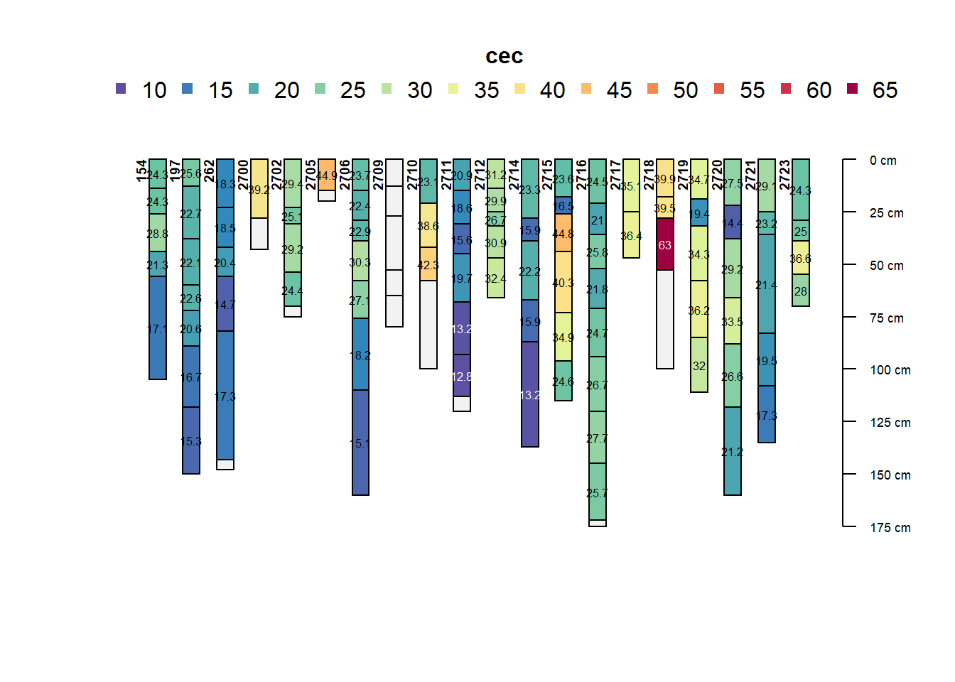
## 4.4 - check data integrity -----------------------------------
# A valid profile is TRUE if all of the
# following criteria are false:
#    + depthLogic : boolean, errors related to depth logic
#    + sameDepth : boolean, errors related to same
#    top/bottom depths
#    + missingDepth : boolean, NA in top / bottom depths
#    + overlapOrGap : boolean, gaps or overlap
#    in adjacent horizons
head(aqp::checkHzDepthLogic(profiles))
## ProfID valid depthLogic sameDepth missingDepth overlapOrGap
## 1 154 TRUE FALSE FALSE FALSE FALSE
## 2 197 TRUE FALSE FALSE FALSE FALSE
## 3 262 TRUE FALSE FALSE FALSE FALSE
## 4 2700 TRUE FALSE FALSE FALSE FALSE
## 5 2702 TRUE FALSE FALSE FALSE FALSE
## 6 2705 TRUE FALSE FALSE FALSE FALSE# Identify non-valid profiles
dl <- checkHzDepthLogic(profiles)
dl[dl$depthLogic==T | dl$sameDepth==T |
dl$missingDepth==T | dl$overlapOrGap==T,"ProfID"]## [1] 6566 7410 8002If there are profiles that violate the depth logic rules (i.e. overlapping horizons), they can be selected and checked through the Profile ID. In the following step, only profiles with valid horizon logic are selected. Finally, the soil profile collection is re-converted to a dataframe. With this, the quality check is finished.
# visualize some of these profiles by the pid
subset(profiles, grepl(6566, ProfID, ignore.case = TRUE))
## SoilProfileCollection with 1 profiles and 4 horizons
## profile ID: ProfID | horizon ID: hzID
## Depth range: 80 - 80 cm
##
## ----- Horizons (4 / 4 rows | 10 / 10 columns) -----
## ProfID hzID top bottom HorID ph k soc bd cec
## 6566 643 0 16 29463 9.4 1.5 2.02 NA 14.0
## 6566 644 16 25 29464 9.5 1.2 0.91 NA 13.0
## 6566 645 26 55 29465 9.1 2.6 0.42 NA 22.7
## 6566 646 55 80 29466 9.0 2.2 0.19 NA 18.8
##
## ----- Sites (1 / 1 rows | 3 / 3 columns) -----
## ProfID x y
## 6566 -58.20125 -37.92759
##
## Spatial Data:
## [EMPTY]subset(profiles, grepl(6915, ProfID, ignore.case = TRUE))## SoilProfileCollection with 1 profiles and 7 horizons
## profile ID: ProfID | horizon ID: hzID
## Depth range: 140 - 140 cm
##
## ----- Horizons (6 / 7 rows | 10 / 10 columns) -----
## ProfID hzID top bottom HorID ph k soc bd cec
## 6915 864 0 6 31278 6.0 2.8 15.78 NA 46.6
## 6915 865 6 14 31279 6.7 1.8 5.65 NA 31.8
## 6915 866 14 21 31280 7.5 0.9 2.02 NA 17.3
## 6915 867 21 35 31281 7.6 1.0 0.45 NA 9.1
## 6915 868 35 65 31282 8.2 2.3 0.41 NA 29.7
## 6915 869 65 87 31283 8.5 2.7 0.23 NA 33.1
## [... more horizons ...]
##
## ----- Sites (1 / 1 rows | 3 / 3 columns) -----
## ProfID x y
## 6915 -58.23173 -37.59698
##
## Spatial Data:
## [EMPTY]subset(profiles, grepl(7726, ProfID, ignore.case = TRUE))## SoilProfileCollection with 1 profiles and 5 horizons
## profile ID: ProfID | horizon ID: hzID
## Depth range: 155 - 155 cm
##
## ----- Horizons (5 / 5 rows | 10 / 10 columns) -----
## ProfID hzID top bottom HorID ph k soc bd cec
## 7726 1581 0 27 35695 6.5 1.2 19.00 NA 27.0
## 7726 1582 27 38 35696 6.6 1.4 1.97 NA 24.8
## 7726 1583 38 70 35697 6.9 1.4 0.83 NA 29.7
## 7726 1584 70 97 35698 7.2 1.4 0.20 NA 18.0
## 7726 1585 97 155 35699 7.3 1.2 NA NA 13.8
##
## ----- Sites (1 / 1 rows | 3 / 3 columns) -----
## ProfID x y
## 7726 -58.8281 -37.32196
##
## Spatial Data:
## [EMPTY]## 4.5 - keep only valid profiles -------------------------------
clean_prof <- HzDepthLogicSubset(profiles)## dropping profiles with invalid depth logic, see `metadata(x)$removed.profiles`metadata(clean_prof)$removed.profiles## [1] 6566 7410 8002# write_rds(clean_prof, "01-Data/soilProfileCollection.rds")
## 4.6 convert soilProfileCollection to a table -----------------
dat <- left_join(clean_prof@site, clean_prof@horizons)## Joining with `by = join_by(ProfID)`dat <- select(dat, ProfID, HorID, x, y, top, bottom, ph:cec )6.3 Calculation of pedo-transfer functions
In the cases of single-layer samples, which is common in sampling for nutrient determination, a locally calibrated pedotransfer function (PTF) should be applied. PTF will be also required to harmonise the laboratory methods. Experts from the Global Soil Laboratory Network (GLOSOLAN) will provide advice in this regard.
Therefore, a customised function is introduced to our working environment. Users can write their own functions in R. This is often necessary when existing functions need to be customised or very specific calculations need to be performed. Functions greatly increase the efficiency of our code. For further information, it is recommendable to consult online resources on the topic (e.g. https://hbctraining.github.io/Intro-to-R/lessons/03_introR-functions-and-arguments.html).
The function estimateBD below calculates various PTFs that estimate bulk density (BD). Which equation is used is determined by the user that has to choose one of the methods and also specify the SOC value of the respective horizon. The SOC values is first converted to OM by using the conversion factor of 1.724 and then inserted in the respective PTF. The return() command tells R which value to output.
# 5 - Estimate BD using pedotransfer functions ==================

# create the function with all PTF
method_names <- c("Saini1996", "Drew1973", "Jeffrey1979",
                  "Grigal1989",
                  "Adams1973", "Honeyset_Ratkowsky1989")

estimateBD <- function(SOC=NULL, method=NULL) {
  OM <- SOC * 1.724
  BD <- switch(method,
           "Saini1996" = 1.62 - 0.06 * OM,
           "Drew1973" = 1 / (0.6268 + 0.0361 * OM),
           "Jeffrey1979" = 1.482 - 0.6786 * (log(OM)),
           "Grigal1989" = 0.669 + 0.941 * exp(1)^(-0.06 * OM),
           "Adams1973" = 100 / (OM / 0.244 + (100 - OM) / 2.65),
           "Honeyset_Ratkowsky1989" = 1 / (0.564 + 0.0556 * OM),
           stop("Invalid method specified.")
  )
  return(BD)
}
To apply the estimateBD function, first a test dataframe is created that includes the SOC values from the cleaned profile table as well as the respective existing BD measurements. The rows without values in one of the columns are excluded using the na.omit() function since we want to first evaluate the difference between estimated BDs and measured BDs.
Now, the test dataframe is complemented by the estimated BDs derived from the PTFs for each method. To add new columns to an existing dataframe one has to write on the left-hand side of the arrow the name of the existing dataframe object (in this case BD_test), the dollar sign ($), and the name of the new column. Here, the names are given according to the used BD PTF.
## 5.1 - Select a pedotransfer function -------------------------
# Create a test dataset with BD and SOC data
BD_test <- data.frame(SOC = dat$soc, BD_observed = dat$bd)

# Remove missing values
BD_test <- BD_test[complete.cases(BD_test),]
BD_test <- na.omit(BD_test)


# 5.2 - Estimate BLD for a subset using the pedotransfer function
for (i in method_names) {
  BD_test[[i]] <- estimateBD(BD_test$SOC, method = i)
}

# Print the resulting data frame
BD_test
## SOC BD_observed Saini1996 Drew1973 Jeffrey1979 Grigal1989 Adams1973
## 367 1.64 1.16 1.450358 1.371991 0.7767016 1.463173 2.072261
## 373 2.38 1.26 1.373813 1.290451 0.5239880 1.404651 1.886665
## 374 0.50 1.49 1.568280 1.519946 1.5827721 1.562569 2.442399
## 376 2.05 1.14 1.407948 1.325584 0.6252763 1.430196 1.965153
## 377 0.44 1.36 1.574486 1.528622 1.6695198 1.568132 2.465577
## 386 0.75 1.43 1.542420 1.484831 1.3076235 1.539757 2.350336
## 387 0.75 1.38 1.542420 1.484831 1.3076235 1.539757 2.350336
## 389 3.20 0.87 1.288992 1.210718 0.3230883 1.344826 1.716329
## 394 1.11 1.25 1.505182 1.437024 1.0415837 1.507928 2.229331
## Honeyset_Ratkowsky1989
## 367 1.386576
## 373 1.262414
## 374 1.634181
## 376 1.314922
## 377 1.649686
## 386 1.572597
## 387 1.572597
## 389 1.148456
## 394 1.491650The calculated BDs can now be compared using the summary() function. However, a faster and more accessible approach is to plot the different bulk densities for comparison. In case you are not familiar with the plot() function and its respective commands, it is recommendable to check one of the many online learning resources such as https://intro2r.com/simple-base-r-plots.html. The plot shows us both measured and estimated BD values as differently coloured lines.
## 5.3 Compare results ------------------------------------------

# Observed values:
summary(BD_test)
## SOC BD_observed Saini1996 Drew1973
## Min. :0.440 Min. :0.87 Min. :1.289 Min. :1.211
## 1st Qu.:0.750 1st Qu.:1.16 1st Qu.:1.408 1st Qu.:1.326
## Median :1.110 Median :1.26 Median :1.505 Median :1.437
## Mean :1.424 Mean :1.26 Mean :1.473 Mean :1.406
## 3rd Qu.:2.050 3rd Qu.:1.38 3rd Qu.:1.542 3rd Qu.:1.485
## Max. :3.200 Max. :1.49 Max. :1.574 Max. :1.529
## Jeffrey1979 Grigal1989 Adams1973 Honeyset_Ratkowsky1989
## Min. :0.3231 Min. :1.345 Min. :1.716 Min. :1.148
## 1st Qu.:0.6253 1st Qu.:1.430 1st Qu.:1.965 1st Qu.:1.315
## Median :1.0416 Median :1.508 Median :2.229 Median :1.492
## Mean :1.0176 Mean :1.485 Mean :2.164 Mean :1.448
## 3rd Qu.:1.3076 3rd Qu.:1.540 3rd Qu.:2.350 3rd Qu.:1.573
## Max. :1.6695 Max. :1.568 Max. :2.466 Max. :1.650# Compare data distributions for observed and predicted BLD
plot.bd <- BD_test %>%
select(-SOC) %>%
pivot_longer(cols = c("BD_observed", "Saini1996", "Drew1973",
"Jeffrey1979",
"Grigal1989", "Adams1973",
"Honeyset_Ratkowsky1989"),
names_to = "Method", values_to = "BD") %>%
ggplot(aes(x = BD, color = Method)) +
geom_density()
plot.bd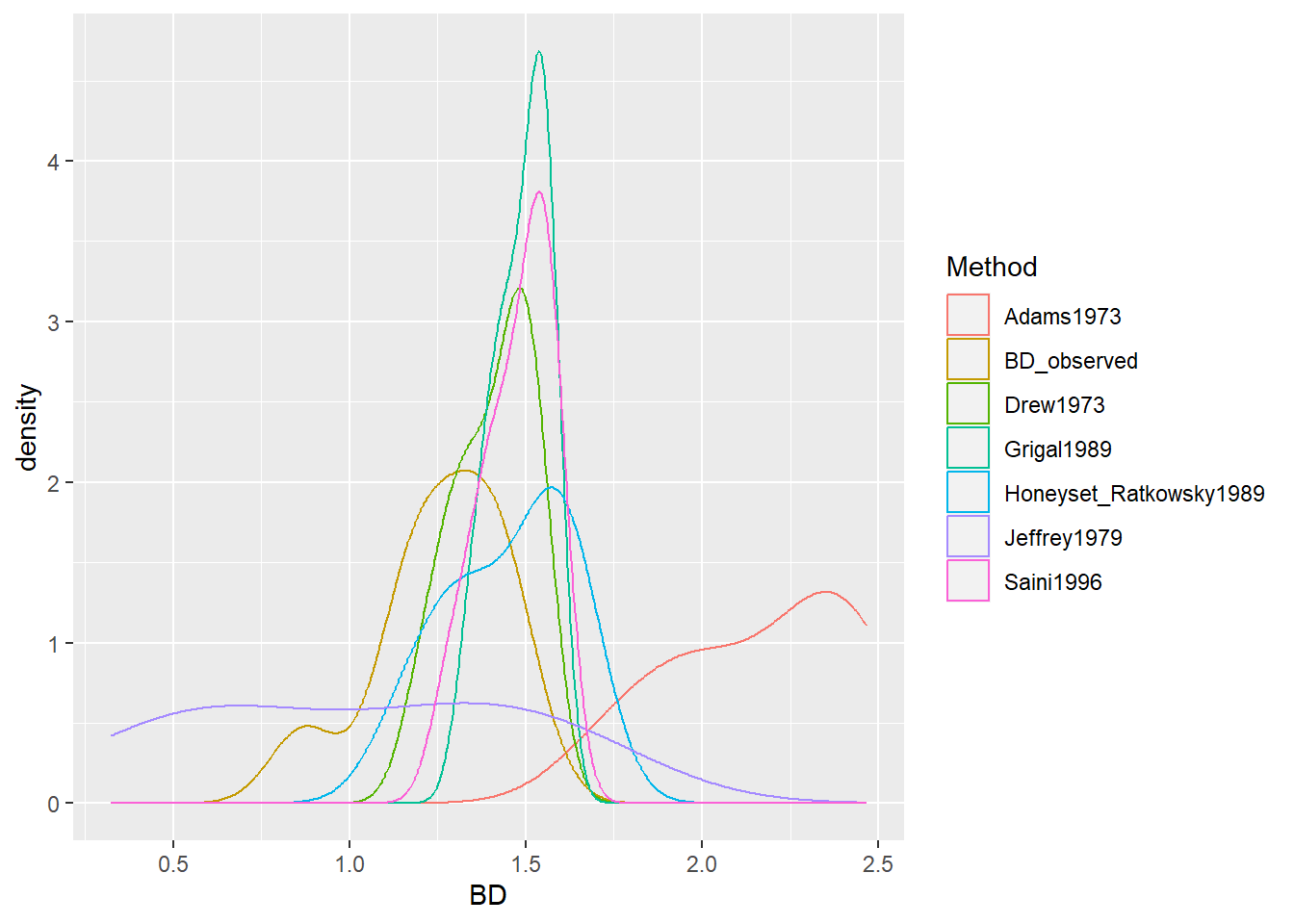
# Dymanic plot with plotly
plotly::ggplotly(plot.bd)plotly::ggplotly(plot.bd) # Plot the Selected function again
BD_test %>%
select(-SOC) %>%
pivot_longer(cols = c("BD_observed", "Honeyset_Ratkowsky1989"),
names_to = "Method", values_to = "BD") %>%
ggplot(aes(x = BD, color = Method)) +
geom_density() + xlim(c(0,2.5))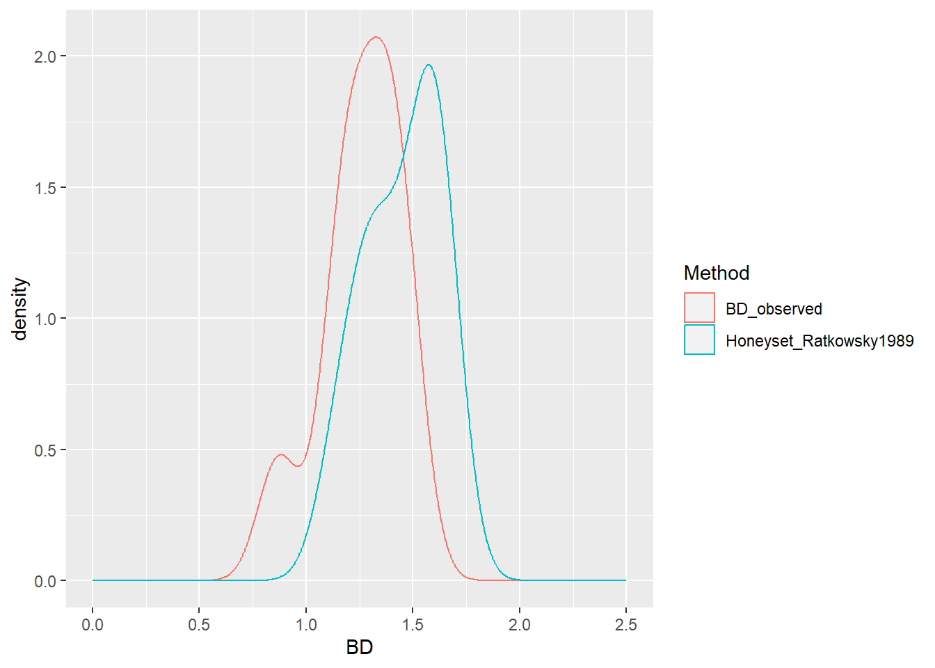
# Same dynamic plot
plotly::ggplotly(BD_test %>%
           select(-SOC) %>%
           pivot_longer(cols = c("BD_observed",
                                 "Honeyset_Ratkowsky1989"),
                        names_to = "Method", values_to = "BD") %>%
           ggplot(aes(x = BD, color = Method)) +
           geom_density() + xlim(c(0,2.5)))
The PTF to be chosen for estimating the BD of the missing horizons should be the closest to the measured BD values. Once, the appropriate PTF was chosen, the estimateBD function is applied in the dataframe dat that was created at the end of the quality check. Here, new bd values are estimated for the rows in which the column ‘bd’ has missing values. Finally, a plot is generated to visualize the gap-filled bulk density values.
## 5.4 Estimate BD for the missing horizons ---------------------
dat$bd[is.na(dat$bd)] <-
estimateBD(dat[is.na(dat$bd),]$soc,
           method="Honeyset_Ratkowsky1989")

# Explore the results
summary(dat$bd)
## Min. 1st Qu. Median Mean 3rd Qu. Max. NA's
## 0.4192 1.2624 1.5797 1.4773 1.7008 1.7670 356g <- BD_test %>%
select(-SOC) %>%
pivot_longer(cols = c("BD_observed"),
names_to = "Method", values_to = "BD") %>%
ggplot(aes(x = BD, color = Method)) +
geom_density() +
xlim(c(0,2.5))
g + geom_density(data = dat, aes(x=bd,
color = "Predicted +\n observed"))## Warning: Removed 356 rows containing non-finite values
## (`stat_density()`).
6.4 Check for outliers
Unrealistically high or low values can have considerable impact on the statistical analysis and thus it is key to identify and carefully check those values in order to get valid results and eliminate potential bias. Again, the summary() function is apt to show general descriptive statistics such as maxima or minima. Based on this assessment, more detailed views of the suspicious values can be obtained by filtering values above or below a certain threshold as done in the code below for soil organic carbon (SOC) values above 10 percent. If such values don’t belong to soil types that would justify such exceptionally high SOC values, e.g. organic soils (Histosols), these rows can be removed based on the profile ID. The same process should be repeated for all soil properties.
Such evaluation can also be conducted visually for several properties at the same time using the tidyverse and ggplot package that allows to plot boxplots for several soil properties at the same time. To get more information on tidyverse, please follow this link: https://r4ds.had.co.nz/. For a comprehensive overview of the functionalities of ggplot, a more sophisticated way of plotting, this book provides a good overview: http://www.cookbook-r.com/Graphs/.
## 5.5 - Explore outliers ---------------------------------------
# Outliers should be carefully explored and compared with
# literature values.
# Only if it is clear that outliers represent impossible
# or highly unlikely
# values, they should be removed as errors.
#
# Carbon content higher than 15% is only typical for organic soil
# (histosols)
# We will remove all atypically high SOC as outliers
summary(dat$soc)
## Min. 1st Qu. Median Mean 3rd Qu. Max. NA's
## 0.020 0.250 0.720 1.451 2.340 19.000 356na.omit(dat$ProfID[dat$soc > 10])## [1] 6915 7726
## attr(,"na.action")
## [1] 1 2 3 4 5 6 7 8 9 10 11 12 13 14 15 16 17 18
## [19] 19 20 21 22 23 24 25 26 27 28 29 30 31 32 33 34 35 36
## [37] 37 38 39 40 41 42 43 44 45 46 47 48 49 50 51 52 53 54
## [55] 55 56 57 58 59 60 61 62 63 64 65 66 67 68 69 70 71 72
## [73] 73 74 75 76 77 78 79 80 81 82 83 84 85 86 87 88 89 90
## [91] 91 92 93 94 95 96 97 98 99 100 101 102 103 104 105 106 107 108
## [109] 109 110 111 112 113 114 115 116 117 118 119 120 121 122 124 125 126 127
## [127] 128 129 130 131 132 133 134 135 136 137 138 139 140 141 142 143 144 145
## [145] 146 147 148 149 150 151 152 153 154 155 156 157 158 159 160 161 162 163
## [163] 164 165 166 167 168 169 170 171 172 173 174 175 176 177 178 179 180 181
## [181] 182 183 184 185 186 187 188 189 190 191 192 193 194 195 196 197 198 199
## [199] 200 201 202 203 204 205 206 207 208 209 210 211 212 213 214 215 216 217
## [217] 218 219 220 221 222 223 224 225 226 227 228 229 230 231 232 233 234 235
## [235] 236 237 238 239 240 241 242 243 244 245 246 247 248 249 250 251 252 253
## [253] 254 255 256 257 258 259 260 261 262 263 264 265 266 267 268 269 270 271
## [271] 272 273 274 275 276 277 278 279 280 281 282 283 284 285 286 287 288 289
## [289] 290 291 292 293 294 295 296 297 298 299 300 301 302 303 304 305 306 307
## [307] 308 309 310 311 312 313 314 315 316 317 318 319 320 321 322 323 324 325
## [325] 326 327 328 329 330 331 332 333 334 335 336 337 339 340 341 342 343 344
## [343] 345 346 347 348 349 350 351 352 353 354 355 356 357 358
## attr(,"class")
## [1] "omit"dat$ProfID[dat$soc > 10][!is.na(dat$ProfID[dat$soc > 10])] ## [1] 6915 7726dat <- dat[dat$ProfID != 6915,]
dat <- dat[dat$ProfID != 7726,]
dat<- dat[!(dat$ProfID %in%
dat$ProfID[dat$soc > 10][!is.na(dat$ProfID[dat$soc > 10])]),]
# Explore bulk density data, identify outliers
# remove layers with Bulk Density < 1 g/cm^3
low_bd_profiles <- na.omit(dat$ProfID[dat$bd<1])
dat <- dat[!(dat$ProfID %in% low_bd_profiles),]
# Explore data, identify outliers
x <- pivot_longer(dat, cols = ph:cec, values_to = "value",
names_to = "soil_property")
x <- na.omit(x)
ggplot(x, aes(x = soil_property,
y = value, fill = soil_property)) +
geom_boxplot() +
facet_wrap(~soil_property, scales = "free")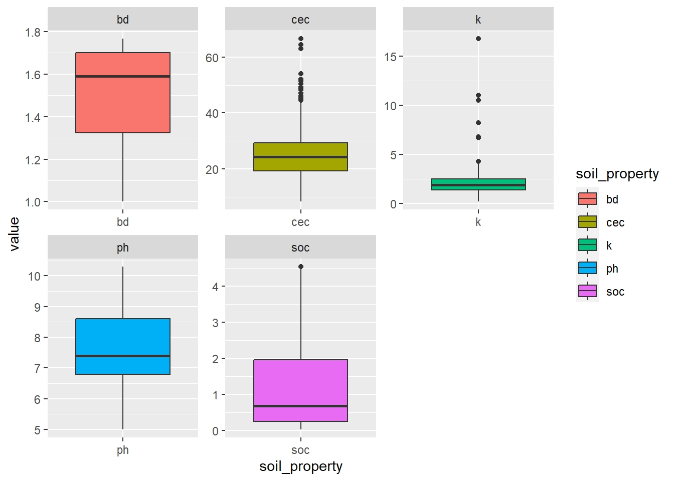
6.5 Harmonise soil layer depths
The last step towards a soil data table that can be used for mapping, is to harmonize the soil depth layers to 0-30 cm (or 30-60, or 60-100 cm respectively). This is necessary since we want to produce maps that cover exactly those depths and do not differ across soil profile locations. Thus, the relevant columns are selected from the dataframe, target soil properties, and upper and lower limit of the harmonised soil layer are specified (in depths).
In the following a new dataframe ‘d’ is created in which the standard depth layers are stored and named. To achieve this the function apply_mpspline_all from mpslpine2 is used.
# 6 - Harmonize soil layers =====================================
source("Digital-Soil-Mapping/03-Scripts/spline_functions.R")
## 6.1 - Set target soil properties and depths ------------------
names(dat)
dat <- select(dat, ProfID, HorID, x, y,
              top, bottom, ph, k, soc, bd, cec)

target <- c("ph", "k", "soc",  "bd", "cec")
depths <- c(0,30)

## 6.2 - Create standard layers ---------------------------------
splines <-apply_mpspline_all(df = dat, properties =
                               target, depth_range = depths)
summary(splines)

# merge splines with x and y
d <- unique(select(dat, ProfID, x, y))
d <- left_join(d, splines)
6.6 Harmonise units
Units are of paramount importance to deliver a high-quality map product. Therefore, special attention needs to be paid to a correct conversion/harmonisation of units particularly if different spreadsheets are combined. The mandatory soil properties need to be delivered in the following units:
# 7 - Harmonise units ===========================================
#Harmonise units if different from target units
# Mandatory Soil Properties and corresponding units:
# Total N - ppm
# Available P - ppm
# Available K - ppm
# Cation exchange capacity cmolc/kg
# pH
# SOC - %
# Bulk density g/cm3
# Soil fractions (clay, silt and sand) -
In the following, the available Potassium measurements from the soil profile data is converted from cmolc/kg to ppm. In addition, total N is converted from percent to ppm and the soil texture class values from g/kg to percent.
# Units soil profile data (dataframe d)
#
head(d) # pH; K cmolc/kg; SOC %; BD g/cm3; CEC  cmolc/kg

# K => convert cmolc/kg to ppm (K *10 * 39.096)
d$k_0_30 <- d$k_0_30*10 * 39.096

head(chem)# P ppm; N %; K ppm
# N => convert % to ppm (N * 10000)
chem$tn <-chem$tn*10000

head(phys)# clay, sand, silt g/kg
# convert g/kg to % (/10)
phys$clay_0_30 <-phys$clay_0_30/10
phys$sand_0_30  <-phys$sand_0_30 /10
phys$silt_0_30 <-phys$silt_0_30/10
Finally, the different spreadsheets are merged into one single dataframe. For that, it is important to have matching column names in the dataframes that are to be merged.
# Add chemical and physical properties from additional datasets =


# Rename columns to match the main data set
names(d)
names(chem)[1] <- 'ProfID'
names(chem)[4] <- 'p_0_30'
names(chem)[5] <- 'k_0_30'
names(chem)[6] <- 'n_0_30'


#The chem dataframe comes from and independent dataset we need to
#create new unique ProfIDs
#Create unique ProfID
chem$ProfID <- seq(max(d$ProfID)+1,max(d$ProfID)+1+nrow(chem)-1)

# Add the new data as new rows using dplyr we can add empty rows
# automatically for the not measured properties in the chem dataset
d <- bind_rows(d, chem)

#The phys dataframe with the texture instead shares the same
#ProfIDs (we can directly merge)
d <- left_join(d, phys, by=c('ProfID', 'x', 'y'))
6.7 Save the results
Before finalising the soil data preparation, it is recommendable to check again visually if the calculations were conducted correctly. Again, the combination of tidyverse and ggplot functions provides high efficiency and versatility to visualise figures with the desired soil properties. At last, the write_csv() function is used to save the dataframe as a .csv file in the Outputs folder (02-Outputs). With this, the soil data preparation is finalised.
# 8 - Plot  and save results ====================================
names(d)
x <- pivot_longer(d, cols = ph_0_30:silt_0_30,
                  values_to = "value",
                  names_sep = "_",
                  names_to = c("soil_property", "top", "bottom"))
x <- mutate(x, depth = paste(top, "-" , bottom))
#x <- na.omit(x)
ggplot(x, aes(x = depth, y = value, fill = soil_property)) +
  geom_boxplot() +
  facet_wrap(~soil_property, scales = "free")


plotly::ggplotly(ggplot(x, aes(x = depth, y = value,
                               fill = soil_property)) +
           geom_boxplot() +
           facet_wrap(~soil_property, scales = "free"))

# save the data
write_csv(d, "02-Outputs/harmonized_soil_data.csv")