 Global Soil Nutrient and Nutrient Budgets maps (GSNmap) Phase I
Annex IV: Quality assurance and quality control
The following protocol was devised to provide National Experts with a step-by-step guideline to perform a Quality Assurance (QA) and Quality Control (QC) of the 10 GSNmap first phase products.
The following protocol does not provide any guidance in terms of uncertainty estimation and validation. For more details and information on the estimation of uncertainties and potential map validation strategies please refer to Chapter 8.4.
Quality assurance and quality control consist of activities to ensure the quality of a particular result. Quality control is a reactive process that focuses on identifying defects and errors while quality assurance is a proactive approach aimed at preventing defects and errors. In the context of digital soil mapping, both processes are often interlinked. A QA is interlinked with a QC when it identifies defects and the QA remodels the process to eliminate the defects and prevent them from recurring (Chapman, 2005)(Figure10.2).
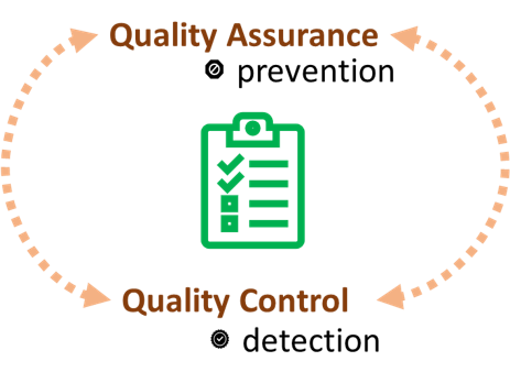
Figure 10.2: Quality assurance and quality control.
Each step in the following protocol should be considered in order to detect and eliminate errors, address data inaccuracies and assess the output completeness.
Step 1: Completeness of layers
The following Table (tab:products) gives an overview of all the GSNmap products in alphabetical order. Each product should include the ISO 3166-1 alpha-3 country code as uppercase letters in its name. For instance, in the case of Turkiye, ISO_GSNmap_Ntot_Map030 should be changed to TUR_GSNmap_Ntot_Map030.
All 10 soil property and soil nutrient maps with their corresponding 10 uncertainty layers must be georeferenced TIF (.tif) files.
| Product | Filename |
|---|---|
| Major nutrients (3 files) | |
| Total Nitrogen map | ISO_GSNmap_Ntot_Map030.tiff |
| Available Phosphorus map | ISO_GSNmap_Pav_Map030.tiff |
| Total Potassium map | ISO_GSNmap_Ktot_Map030.tiff |
| Associated soil properties (7 files) | |
| Cation exchange capacity map | ISO_GSNmap_CEC_Map030.tiff |
| Soil pH map | ISO_GSNmap_pH_Map030.tiff |
| Soil clay map | ISO_GSNmap_Clay_Map030.tiff |
| Soil silt map | ISO_GSNmap_Silt_Map030.tiff |
| Soil sand map | ISO_GSNmap_Sand_Map030.tiff |
| Soil organic carbon map | ISO_GSNmap_SOC_Map030.tiff |
| Soil bulk density map | ISO_GSNmap_BD_Map030.tiff |
| Uncertainty maps (10 files) | |
| Total Nitrogen uncertainty map | ISO_GSNmap_Ntot_UncertaintyMap030.tiff |
| Available Phosphorus uncertainty map | ISO_GSNmap_Pav_UncertaintyMap030.tiff |
| Total Potassium uncertainty map | ISO_GSNmap_Ktot_UncertaintyMap030.tiff |
| Cation exchange capacity uncertainty map | ISO_GSNmap_CEC_UncertaintyMap030.tiff |
| Soil pH uncertainty map | ISO_GSNmap_pH_UncertaintyMap030.tiff |
| Soil clay uncertainty map | ISO_GSNmap_Clay_UncertaintyMap030.tiff |
| Soil silt uncertainty map | ISO_GSNmap_Silt_UncertaintyMap030.tiff |
| Soil sand uncertainty map | ISO_GSNmap_Sand_UncertaintyMap030.tiff |
| Soil organic carbon uncertainty map | ISO_GSNmap_SOC_UncertaintyMap030.tiff |
| Soil bulk density uncertainty map | ISO_GSNmap_BD_UncertaintyMap030.tiff |
Step 2: Check the projection and resolution of all data products
Open the products in QGIS or any other preferred GIS platform. Check that the projection of all products is EPSG:4326 - WGS 84 (Layer properties). Check that the spatial resolution (pixel size) (Layer properties) is equal to ~0.002246 degrees ; 250 m x 250 m at the equator.
Step 3: Check the extent
Visualize the 20 products in QGIS or any preferred GIS platform. Load a land-use layer to visually assess that the simulations were done exclusively on croplands.
Step 4: Check the units, ranges, and outliers
In the following section possible value ranges for each product category (except available potassium) are presented. It is important to note that the provided ranges represent a gross approximation of the extremes within which the values should fall in. Results that fall outside these ranges need to be carefully evaluated based on local expertise and available literature.
The provided ranges can be compared in QGIS, R, or any preferred platform. Descriptive layer statistics can be viewed in QGIS under Layer Properties.
The following table (Table 10.2) presents ranges of possible values for 9 of the 10 mandatory GSNmap products. The ranges were calculated based on the distribution of the soil profile data within the World Soil Information Service (WoSIS), specifically the WoSIS snapshot 2019 (Batjes, N. H. et al. 2020). It is important to note that the data was not filtered for croplands and that the ranges were extracted from soil profiles sampled globally from a wide array of land covers and land uses.
| Soil property | property_id | Unit | Min | 1st Quartile | Median | 3st Quartile | Max | n |
|---|---|---|---|---|---|---|---|---|
| Total N | n_0_30 | ppm | 0.0 | 400.0 | 700.0 | 1500.0 | 84000.0 | 216362 |
| P Bray I | p_0_30 | ppm | 0.0 | 1.6 | 5.0 | 16.0 | 150.0 | 40486 |
| P Mehlich 3 | p_0_30 | ppm | 0.0 | 1.6 | 6.1 | 22.0 | 149.4 | 7242 |
| P Olsen | p_0_30 | ppm | 0.0 | 0.7 | 2.0 | 4.3 | 141.0 | 8434 |
| CEC | cec_0_30 | cmol(c)/kg | 0.1 | 7.5 | 14.0 | 23.0 | 140.0 | 295688 |
| pH (water) | ph_0_30 | / | 1.5 | 5.2 | 6.2 | 7.5 | 12.3 | 613322 |
| Clay | clay_0_30 | % | 0.0 | 11.1 | 21.9 | 35.3 | 100.0 | 590368 |
| Silt | silt_0_30 | % | 0.0 | 15.0 | 30.0 | 47.6 | 100.0 | 558233 |
| Sand | sand_0_30 | % | 0.0 | 15.0 | 36.0 | 60.2 | 100.0 | 482334 |
| Soil Organic Carbon | soc_0_30 | % | 0.0 | 2.0 | 5.1 | 14.0 | 99.4 | 471301 |
| Bulk density | bd_0_30 | g/cm3 | 0.0 | 1.3 | 1.4 | 1.7 | 2.6 | 116756 |
| Available K | k_0_30 | ppm | NA | NA | NA | NA | NA | NA |
QA/QC Script
The following script automates the for Steps described in the previous sections. It is important to note that the script’s main objective is to provide a fast alternative to check the output layers and that it does not replace the need to visually assess the final maps based on expert knowledge.
#_______________________________________________________________________________
#
# QA/QC
# Soil Property Mapping
#
# GSP-Secretariat
# Contact: Isabel.Luotto@fao.org
#          Marcos.Angelini@fao.org
#_______________________________________________________________________________

#Empty environment and cache
rm(list = ls())
gc()

# Content of this script =======================================================
# 0 - Set working directory and packages
# 1 - Step 1: Completeness of layers
# 2 - Step 2: Check the projection and resolution of all data products
# 3 - Step 3: Check the extent
# 4 - Step 4: Check the units, ranges, and outliers
#
# 5 - Export QA/QC report
#_______________________________________________________________________________


# 0 - Set working directory, soil attribute, and packages ======================

# Working directory
wd <- 'C:/Users/hp/Documents/GitHub/GSNmap-TM/Digital-Soil-Mapping'
#wd <- 'C:/Users/luottoi/Documents/GitHub/GSNmap-TM/Digital-Soil-Mapping'
setwd(wd)

# Define country of interes throuhg 3-digit ISO code
ISO ='ISO'

#load packages
library(terra)
library(readxl)

# Load reference values
dt <- read_xlsx("C:/Users/luottoi/Documents/GitHub/GSNmap-TM/tables/wosis_dist.xlsx")
dt <- dt[!(dt$`Soil property` %in%c( "P Bray I","P Olsen" )),]

# In case old naming system was used
dt$old_prop_ids <- c('Ntot', 'Pav', 'CEC','pH', 'Clay', 'Silt', 'Sand', 'SOC', 'BD', 'Kav')


## Set potential ranges for Available K in ppm

dt[dt$property_id=='k_0_30','Min'] <- 0
dt[dt$property_id=='k_0_30','Max'] <- 150
# 1 - Step 1: Completeness of layers -------------------------------------------

#Check number of layers

## Specify number of soil property maps generated (not including the uncertainty layers)

## Check if all layers were correctly generated (including uncertainty layers)
# and if the correct ISO code and soil property ids were included in the files names
files <- list.files(pattern= '.tif', full.names = T)
names <- list.files( pattern= '.tif', full.names = F)
names <- sub('.tif', '', names)


# Switch depending on the naming system (i.e. files have e.g. Pav instead of p_0_30)
#Step1 <-data.frame(property_id =dt$property_id)
Step1 <-data.frame(property_id =dt$old_prop_ids) #old naming system

Step1$Names <- 'Rename layer'
Step1$Uncertainty <- 'Missing'

for (i in unique(Step1$property_id)){

  t11 <- TRUE %in% grepl(paste0('SD_GSNmap_',i), files)|grepl(paste0('sd_',i), files)
  t12 <- TRUE %in% grepl(paste0(ISO,'_GSNmap_',i), files)|grepl(paste0('mean_',i), files)

  t13 <- TRUE %in% grepl(ISO, files)

  Step1[Step1$property_id ==i, 'Names'] <- ifelse(t12[[1]] ==T & t13[[1]] ==T, 'Correctly named', 'Rename layer')
  Step1[Step1$property_id ==i, 'Uncertainty'] <- ifelse(t11[[1]] ==T , 'Generated', 'Missing')

}


# 2 - Step 2: Check the projection and resolution of all data products ---------
r <- rast(files)
names(r) <- names
# Check projection (WGS 84)
(Step21=crs(r, describe=TRUE)$name =='WGS 84')

# Check resolution (250 m)
(Step22=round(res(r)[[1]], 5) == 0.00225)

# 3 - Step 3: Check the extent -------------------------------------------------
# Check if the layers were masked with a cropland mask

mask <- rast('mask/mask.tif')
mask <- project(mask, r[[1]])

t <- r[[1]]
t <- ifel(!is.na(t),1, NA)

t3 <- sum(values(t, na.rm=T))-sum(values(mask, na.rm=T))

(Step3= t3 <=10)


# 4 - Step 4: Check the units, ranges, and outliers ----------------------------
Step4 <- data.frame(property_id=Step1$property_id)
#Step4 <- data.frame(property_id =dt$property_id)
Step4$in_range <- 'Values not in range'

for (i in unique(Step4$property_id)){
  t41 <-min(values(r[[grepl(paste0('mean_',i), names(r))|grepl(paste0(ISO,'_GSNmap_',i), names(r))]],na.rm=T)) >=dt[Step4$property_id == i, 'Min']
  t42 <-max(values(r[[grepl(paste0('mean_',i), names(r))|grepl(paste0(ISO,'_GSNmap_',i), names(r))]],na.rm=T)) <=dt[Step4$property_id == i, 'Max']

  Step4[Step4$property_id ==i, 'in_range'] <- ifelse(t41[[1]] ==T & t42[[1]] ==T, 'Values in range', 'Values not in range')

}


# 5 - Export QA/QC report ------------------------------------------------------
report <- merge(Step4, Step1, by=c('property_id'))

report$projection <- ifelse(Step21, 'WGS 84', 'Reproject layer')
report$resolution <- ifelse(Step21, '250 m', 'Resample layer')
report$extent <- ifelse(Step3, 'Croplands', 'Mask out layer')

report

write.csv(report, paste0('QA_QC_', ISO, '.csv'))