Chapter 3 Methods for mapping salt-affected soils

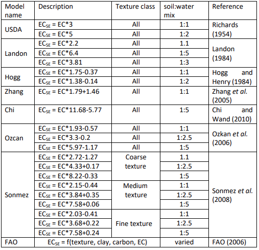
Maps of salt-affected soils contain spatial information of the distribution of types and intensity of salt problems in the soils. They are developed by considering the drivers, indicators, prevalence of salt-affected soils in the landscape and mapping tools and resources (Figure 3.1). Input data on the drivers and indicators provide the evidence of occurrence of salt problems in the soil. They influence the type of mapping tools for information mining and representation of the final maps. Some of the commonly used mapping tools include Geographic Information Systems (GIS), statistical modelling, stereoscopes, etc. Besides the input data and mapping tools, mapping methods are also influenced by resource requirements such as expertise, computing facility, and funding.

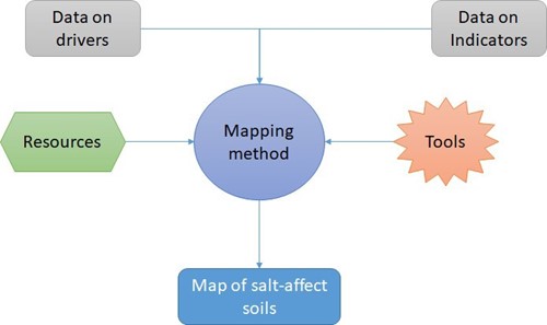
Figure 3.1: Framework for developing mapping methods for salt-affected soils

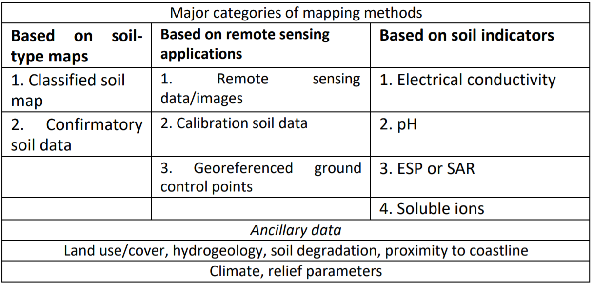
The main categories of the methods for mapping salt-affected soils are:

1. Methods based on soil maps and expert opinion;
2. Remote sensing applications;
3. Modelling of soil indicators of salt problems.

This chapter elaborates on the potential and limitations of these categories of mapping methods with regards to their: 1) contribution to building integral global information of salt-affected soils, 2) ability to quantify mapping accuracy and uncertainty, and 3) flexibility for periodic information update.

3.1 Methods based on soil maps and expert opinion

Soil maps have been traditionally used to identify salt-affected soils in many territories of the world. Their application relies on identification and verification of the areas in the soil maps with designations related to salt-affected soils. A seminal work in global assessment of salt-affected soils using this approach was published by Szabolcs (1979). The publication used FAO-UNESCO soil map of the world in which the polygons with salt-affected soils were classified saline soils (solonchak and saline phases), alkali soils (solonetz and alkaline phases), and potentially salt-affected soils. Potentially salt-affected soils were soils in areas that were not salt-affected at the time (or salt-affected to a very low degree) but could be easily become affected due to human activities. The approach given by Szabolcs (1979) also used expert opinion to identify the areas that were not very well represented in the FAO-UNESCO soil map of the world. Figure 3.2 is example output from this mapping approach.

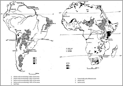
Figure 3.2: Example map of salt-affected soils (adapted from Szabolcs, 1979)

Application of soil maps to quantify areas of salt-affected soils has since been applied in various parts of the world. Examples include mapping of saline and sodic soils in the European Union (Toth et al., 2008), salt-affected soils in the European part of Russia (Khitrov et al., 2009), digital assessment of salt-affected soils in India (Mandal et al., 2011), among others. Most applications of soil maps use the sequence of identification, verification, and quantification processes to produce the spatial information of salt-affected soils. The identification process aims at locating the soil

typological/mapping units in the soil map with classified designations of salt-affected soils. The identified units are then verified with either through expert opinion or confirmatory field-sampling and testing. The confirmed areas are finally delineated and their aerial extent quantified. This sequence may be preceded with the development of a new soil map or digitalization of old maps where necessary (Khitrov et al., 2009; Mandal et al., 2011). Although the application of soil maps to identify salt-affected soils is popular in some countries, it suffers from the lack of accuracy and uncertainty quantification of the final maps. The approach also produces maps of salt-affected soils with hard boundaries, which are arguably infrequent in most landscapes. Other soil information associated with salt-affected soils such as the distribution of electrical conductivity, pH, soluble ions, etc. may be imprecisely given or missing.

3.2 Using remote sensing application

Remote sensing application has been used in agriculture and environment for many years. The technology provides spatial and temporal information about the land cover, soil cover characteristics, climate, and atmospheric conditions, which are of importance in soil and agriculture resources management. It relies on the interaction of the electromagnetic radiations with soil and vegetation to produce characteristic signatures in the reflected radiations. The reflected signatures are then modelled to extract soil and vegetation features. Two broad categories of radiations are discernible with this technology: radiations from the sun (also called passive radiations) or radiations from the sensor (active radiation). They are further classified according to the type of sensors detecting the radiations: 1) proximal sensors, which are put on the soil surface or a few meters from the soil surface; 2) sub-atmosphere cameras, which are carried by low lying aircrafts or aerial vehicles; and 3) satellites (Figure 3.3).

Figure 3.3: Framework for remote sensing of land surface

Remote sensing applications in mapping salt-affected soils target land surface evidence of salt problems in the soil. Examples of proximal sensors often used are electromagnetic induction (EMI), geophysical sounding, and reflectometers. These sensors are mostly used to determine bulk soil electrical conductivity (Lesch et al., 1992). Low-altitude sensors such as Unmanned Arial Vehicles (UAV) are also gaining traction in mapping salt-affected soils (Hu et al., 2019; Ivusking et al., 2019). Hu et al. (2019) tested hyperspectral camera mounted on UAV and EMI in mapping salinity and found UAV as the most promising method for high-resolution identification of soil surface salinity characteristics.

Satellite remote sensing are the most popularly used. They cover wide areas in a single scene, which is economical for large-area mapping. Moreover, most satellite images are increasingly becoming freely downloadable and gaining wide applications because of globally tested models and free processing algorithms. Their applications range from interpretation of composite images to modelling the relationships between indices of image reflectance and indicators of salt problems in the soil (Matternicht and Zinc, 2003; Gorji et al., 2019). Widely used remote sensing images for mapping soil resources are Landsat, sentinel and (Moderate Resolution Imaging Spectroradiometer (MODIS) (Table 3.1). These images are globally available for free download.

Table 3.1: Commonly used remote sensing image characteristics for mapping salt-affected soils

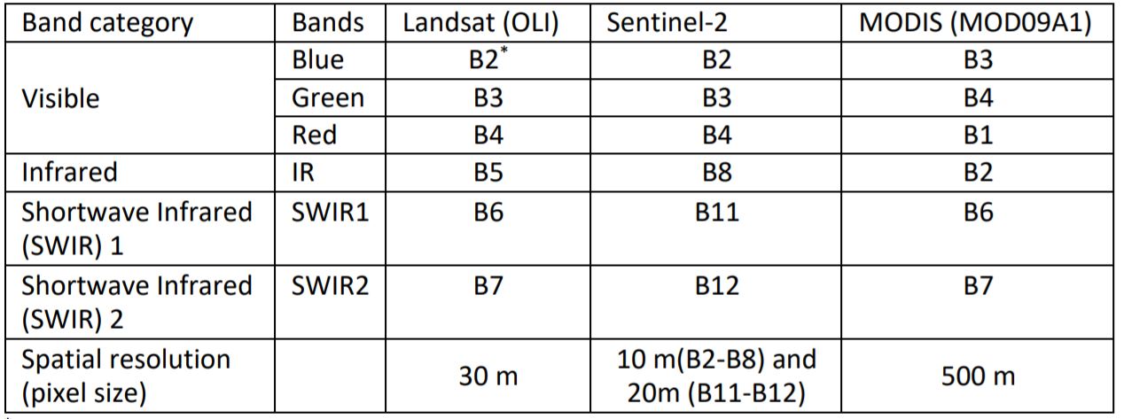
*B is notation for satellite image band
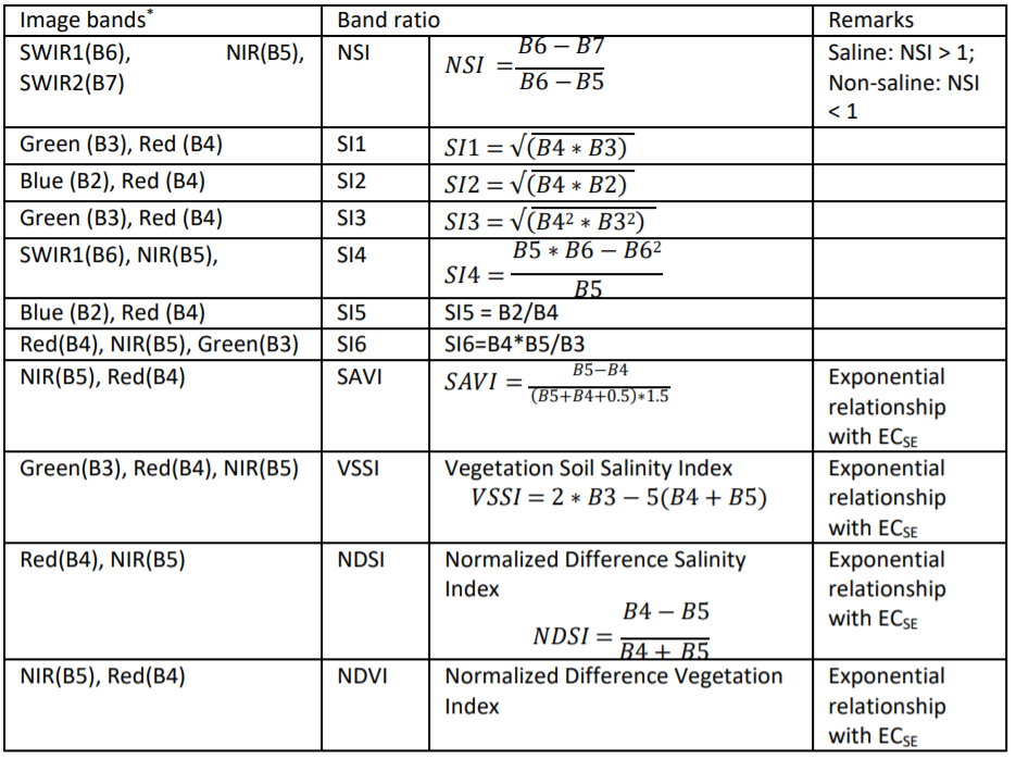
Examples of popularly used image indices in mapping salt-affected soils are normalized salinity index (NSI), salinity index (SI), soil adjusted vegetation index (SAVI), vegetation soil salinity index (VSSI), normalized difference salinity index (NDSI), normalized difference vegetation index (NDVI), salinity ratio (SR), canopy response salinity index (CRSI), and brightness index (BI) (Gorji et al., 2019). They are summarized in Table 3.2. These indices have been variously used either alone or in combination to model soil surface salinity characteristics.

Table 3.2: Examples of popular image band combinations for soil salinity mapping

Remote sensing application for mapping salt-affected soils is expedited by the availability of images and processing software. Consequently, the approach is the fastest of all the methods for mapping salt- affected soils. Its application in large areas often produce consistent maps between boundaries of countries, which minimizes the need for harmonization. Furthermore, its time-series application is potentially useful in monitoring changes in status of salt-affected soils. A recent application at the global level was demonstrated by Ivushkin et al. (2019) (Figure 3.4).

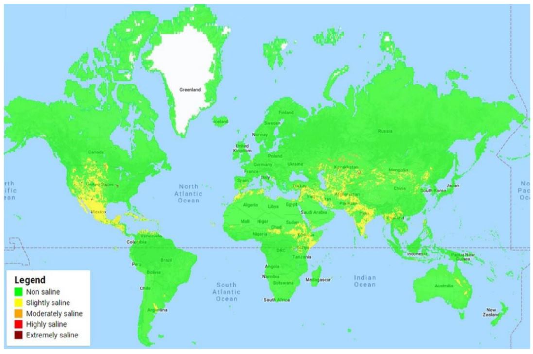
Figure 3.4: Global map of soil salinity using remote sensing applications (source: Ivushkin et al., 2019)

Despite the potential of remote sensing application, the approach is limited in detecting salt problems down the soil profile. Most remote sensing images for large-area mapping do not penetrate more than a few inches of the topsoil and only rely on the calibration models to estimate salt problems down the soil profile. These calibration models can result into spurious relationships without significance in salt dynamics in the soil (Matternicht and Zinc, 2003; Gorji et al., 2019). Some attempts have been made to overcome these limitations. Combined modelling with other spatial datasets such as climate, soil maps and vegetation cover are examples focused on performance improvements of the approach (Scudiero et al., 2019).

3.3 Methods based on soil indicators of salts

Soil indicators provide evidence of the presence of salts in the soil and occurrence of salt-affected soils. They are traditionally used in most soil classification schemes to identify the soil profiles and soil types belonging to the group of salt-affected soil (Soil Survey Staff, 1999; IUSS Working Group WRB, 2015; Craig and Hempel, 2017). Soil indicators of salt-affected soils are also used to quantify the intensity of salt problems in the soil (Table 2.4). They are also used to calibrate other methods for mapping salt-affected soils. Hence, they play a central role in assessing salt-affected soils and should therefore be the foundation for developing soil information of salt-affected soils. Three types of applications exist in the literature for mapping salt-affected soils using soil indicators: 1) mapping the soil attributes and classifying the output maps, 2) mapping classes derived from the soil attributes, and 3) classifying calibrated maps of electromagnetic induction outputs or remote sensing images (Figure 3.5) (Triantafilis et al., 2001; Taghizadeh-Mehrjardi et al., 2019).

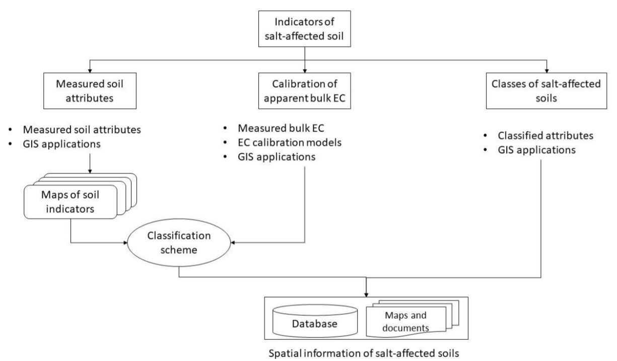
Figure 3.4: Approaches for using soil indicators in mapping salt-affected soils

Applications using calibrated models with EMI are popularly used in mapping soil salinity. In this case, EMI data are calibrated with measured EC on a select sample set and the results used to map soil salinity (Lesch et al., 1992). Farzamian et al. (2019) recently tested the efficacy of local and regional models of this approach to improve its wide adoption. Mapping approaches involving extrapolation of pre-classified classes of salt-affected soils are also available in the literature. These approaches resemble the soil-map based method except that the input data are georeferenced soil attributes. They are not very popular owing to the challenges with extrapolation of categorical attributes (Jafari et al., 2012). Classifying spatially interpolated soil attributes is also another way of mapping salt-affected soils. In this case, the georeferenced soil indicators are first interpolated then the resulting maps are classified into maps of salt- affected soils (Zurqani et al., 2018). This approach was tested by Wicke et al. (2011) to produce a global map of salt-affected soils (Figure 3.6).

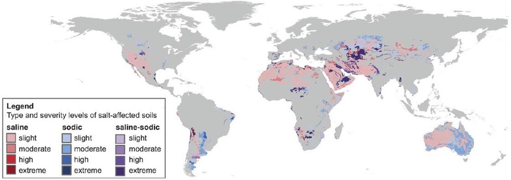
Figure 3.6: Global distribution of salt-affected soils (Source: Wicke et al., 2011)

3.4 Data requirements for mapping soil salinity

Input data for mapping salt-affected soils depends on the mapping methods. A summary of data requirements by the main categories of mapping methods is given in Table 3.3. The soil indicator-based methods are the most data demanding. At least, they require soil data on electrical conductivity (EC), pH, and exchangeable sodium percent (ESP) or sodium adsorption ratio (SAR) as recommended by FAO or USDA classification schemes for salt-affected soils.

Table 3.3: Summary data requirements for mapping salt-affected soils

3.4.1 Measured soil properties

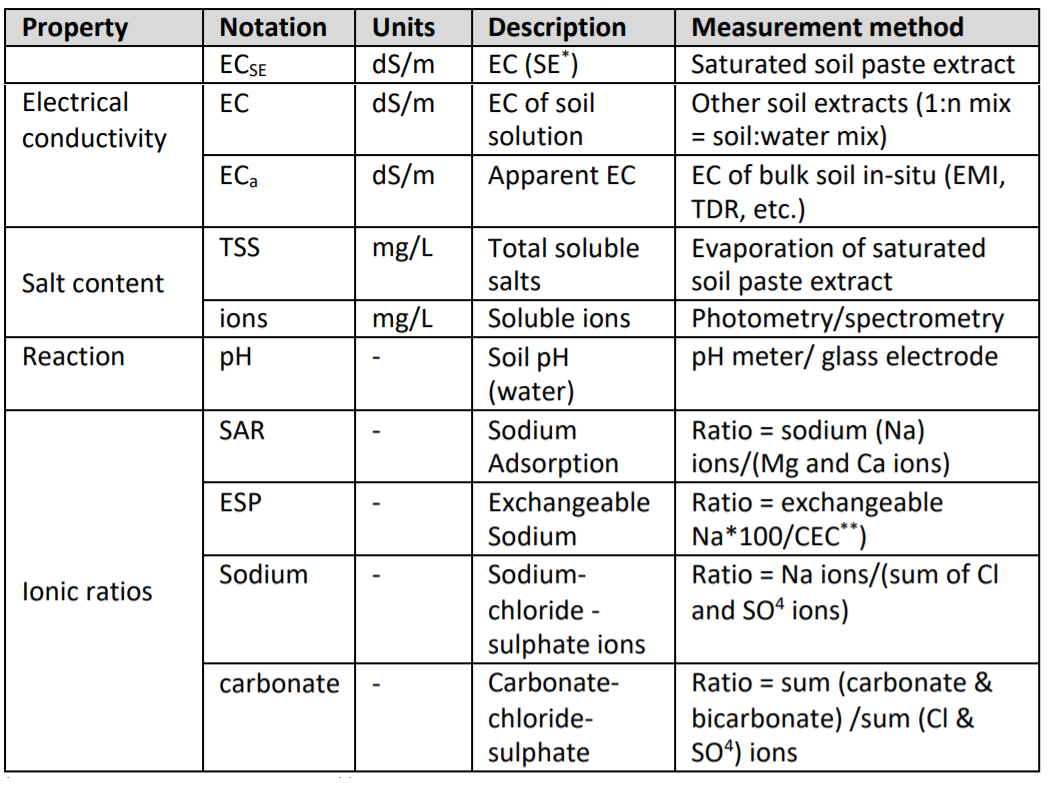
Measured soil properties for classifying salt problems in the soil are given in Table 3.4. Soluble ions in this category include Sodium (Na⁺), Calcium (Ca²⁺), Magnesium (Mg²⁺), Potassium (K⁺), Chloride (Cl^-), Sulphate (SO^-2), Carbonate (CO^-2), Bicarbonate (HCO^-) and Nitrates (NO^-). They are useful in identification of the dominant salts and types of salt-affected soils. Electrical conductivity (EC), total soluble salts (TSS), total soluble cations (TSC), and total dissolved solids (TDS) are integral measures of salt concentration in the soil. This book recommends a minimum data set for classifying salt-affected soils as EC, pH and either ESP or SAR because of the recommendations given by the popular salt classification schemes (Table 2.1). Table 3.4: Summary soil properties for mapping salinity

Table 3.4: Summary soil properties for mapping salinity

3.4.2 Bulk-soil properties and soil maps

Bulk soil properties are properties measured in the field using proximal soil sensors. They are mostly used for estimation of pH and electrical conductivity. The sensors for measuring electrical conductivity are: 1) electrical resistivity, 2) electromagnetic induction, and 3) time domain/amplitude domain/frequency domain reflectometry (TDR, ADR, FDR). They measure electrical conductivity of the bulk soil, which is also known as apparent electrical conductivity (ECa) (Dalton and van Genuchten, 1986; Corwin and Lesch, 2005).

Field measurement of soil pH is often done using pH meters (and sometimes pH sensors). pH meters are used with samples prepared in the field. Hence, they are not really pH of the bulk soil. The sensors for bulk soil pH include field-efficient transistor (ion-selective field efficient transistor - ISFET) and conductimetric sensors, electrode sensors (Schirrmann et al., 2011). Soil maps are ensemble of spatial information of groups (units) of soil with certain characteristics. Typical examples of soil maps are polygon maps showing dominant soil types in each polygon and thematic choropleth maps of indicators/classes of salt-affected soil types.

3.4.3 Information on soil forming factors

Soil forming factors are the parent material, land use/cover, climate, and relief. Information on the parent material is obtained from the geology map. The map should contain data on the age and type of lithology of the dominant rocks from which the soil was formed (Figure 3.7). Most geology maps are available as polygon GIS vector files. Land cover/use information represent the biotic and anthropogenic activities influencing soil formation and secondary drivers of salt problems in the soil. Land cover/cover maps and remote sensing images are suitable sources of information of land cover/use. Examples of climate data are mean annual precipitation (rainfall, snowfall, etc.), annual minimum and maximum temperature, mean annual evapotranspiration rate, and wind speed. Freely downloadable climate data at low-resolution global scale are available at https://www.worldclim.org/ (Accessed on 31 January 2020). Digital elevation model (DEM) is the primary input data for deriving relief information. DEM can be downloadable at https://earthexplorer.usgs.gov/ accessed on 14 January 2020).

3.4.4 Other ancillary data

Other ancillary data for mapping salt-affected soils are administrative boundaries and spatial data of other drivers of salt problems in the soil (Figure 3.7). Spatial data of other drivers of salt problems are maps of hydrogeology (groundwater quality and depth to groundwater level), soil degradation, proximity to coastline, and flood-prone areas.

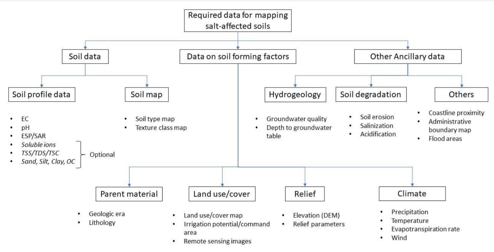
Figure 3.7: Data requirements for mapping salt-affected soils

3.4.5 Conversion models

Electrical conductivity determined on saturated soil paste extract (ECSE in dS/m) is the preferred EC for classifying salt-affected soils. However, many soil laboratories don’t analyse ECSE due to the cumbersome laboratory procedures involved with its determination and long turn-around time for analysing many samples. Instead they use other extracts, such as from 1:5 soil:water mix (1 part of soil in 5 parts of water), 1:2.5 solutions, etc (Landon, 1984). Proposals have been made in the literature to calibrate EC determined from other soil extracts to the ECSE equivalent (Hogg and Henry, 1984, Ozcan et al., 2006; Sonmez et al., 2008; Kargas et al., 2018). These proposals depend on the soil texture, organic matter content, temperature, and measured ECS. A generic framework in these proposals for converting EC to ECSE is as follows:

\[\begin{equation} \tag{3.1} EC_{SE} = f(EC_{s,texture,carbon,temperature}+ \varepsilon ) \end{equation}\]

Table 3.5: Existing EC conversion models