7 Visualization

Two visualization tools are included in this app: a Dashboard viewer and a Data Viewer application in Shiny. Both are designed to display data from the GloSIS database in a user-friendly format, and the Data Viewer also allows the export of soil data points to .csv, .xlsx, and the clipboard.

7.1 View Data on the Dashboard

The first visualization tool is a dashboard generated in .html format. This dashboard is useful for verifying whether the data has been correctly updated in the database, identifying potential errors in positioning, and detecting data outliers. The file contains all selected data from the GloSIS database, which may result in a large file size depending on the number of records.

A Create Dashboard button appears after populating the GloSIS database with soil data (Figure 7.1).

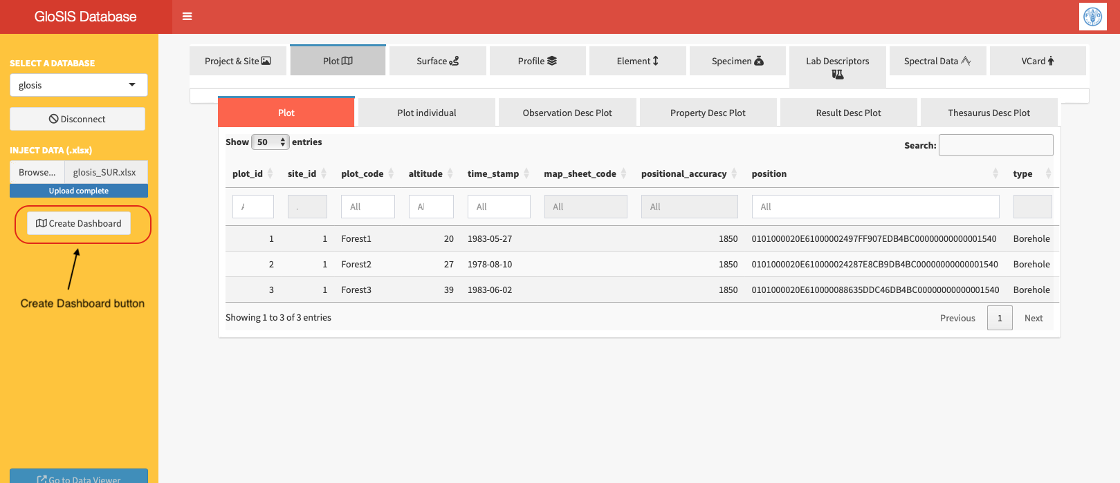
Figure 7.1: Create Dashboard button on the left panel of the data injection app.

Clicking this button generates a .html file stored in the init-scripts folder within the working directory, using the same name as the database. The application then renders the file, and a new button,Go to Dashboard, will appear (Figure 7.2).

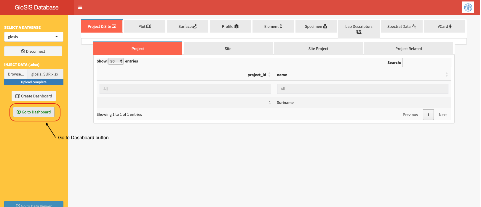
Figure 7.2: Go to Dashboard button in green color.

Clicking this button opens a .htmlformat file in a new tab displaying soil data in three sections (Figure 7.3):

• Location – Contains details about the position of the soil data points.
  
• Attributes – Data on soil properties.
  
• Boxplot – Data with value bars showing the distribution of soil properties across profiles and depths for quick visual comparisons.

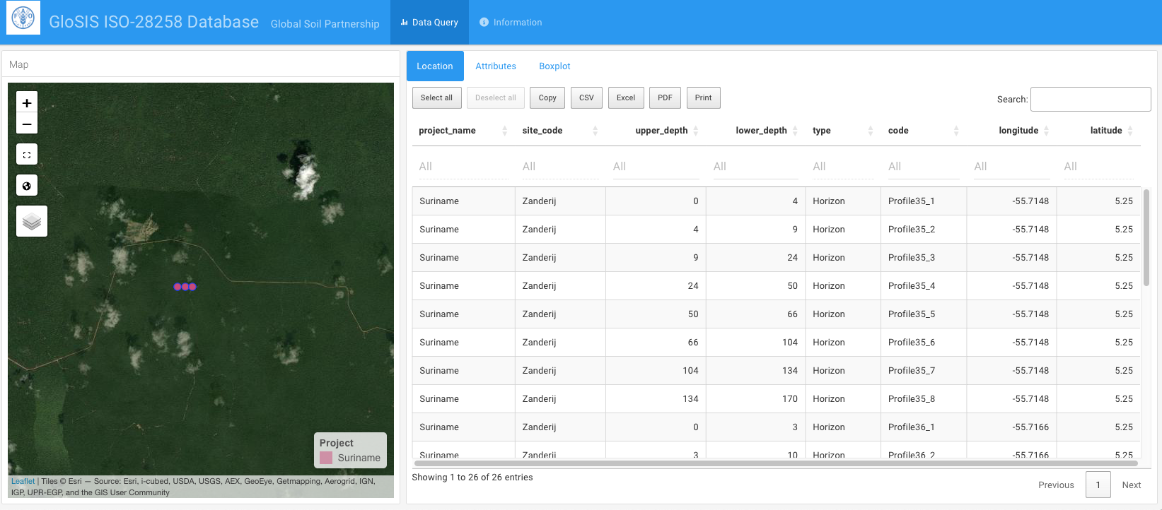
Figure 7.3: Visualization of the soil data in the dashboard..

Tables and the map are internally linked, allowing users to select specific soils either on the map or in the tables, with their location and attributes automatically filtered. The Make a selection button on the map can be used for this task when selecting directly from the map (Figure 7.4).

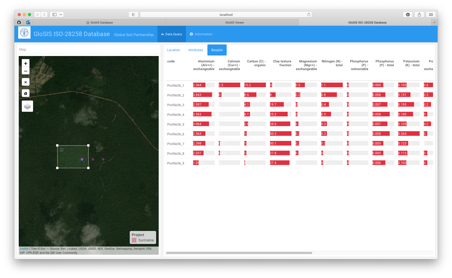
Figure 7.4: Boxplot visualization of filtered soil data attributes.

7.2 View data on the Data Viewer App

The second visualization tool is accessible via the Go to Data Viewer button (Figure 7.5) at the bottom of the glosis-shiny app. Clicking this button opens a new tab (Figure 7.5) with a dropdown menu listing available databases. These databases are those previously created within the glosis-shiny app. The button Go to GloSIS database brings you back to the glosis-shiny app for data injection.

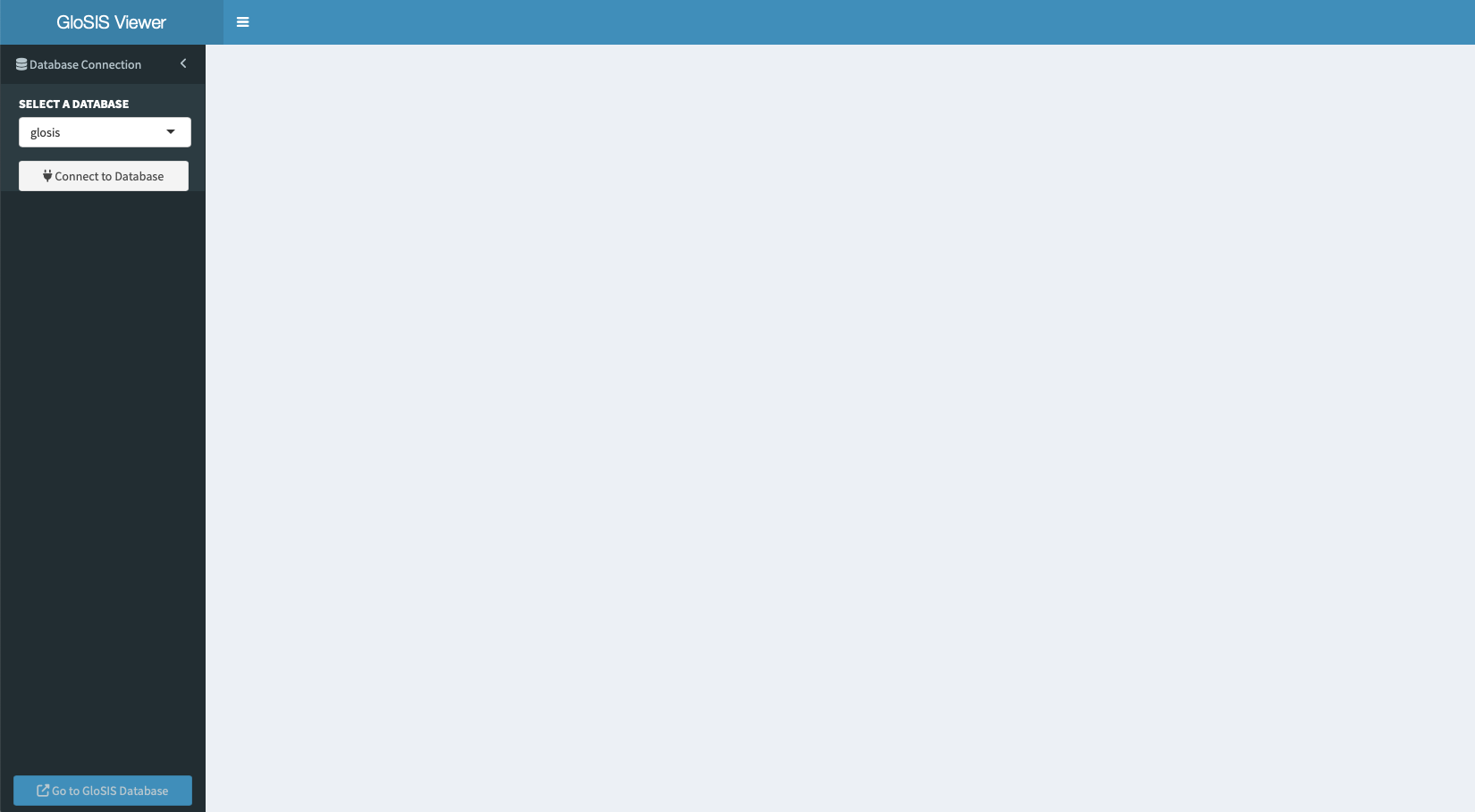
Figure 7.5: Visualization app.

After selecting a database, clicking Connect displays the soil data both in a tabular format and as a map showing the locations of soil samples (Figure 7.6).

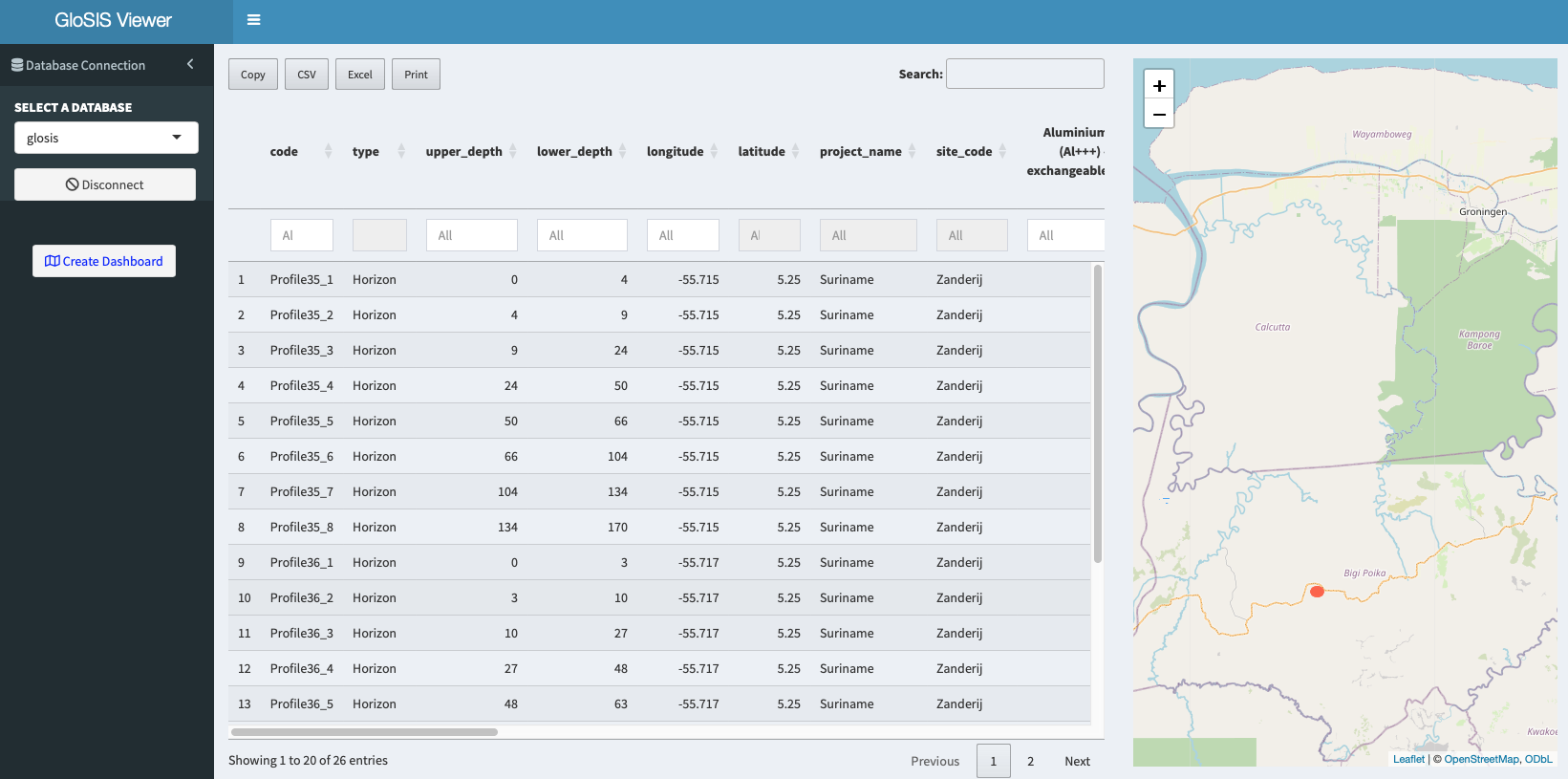
Figure 7.6: Visualization app showing soil data from the selected database.

Similar to the dashboard, this tool is designed primarily for data verification and correction. In this app, soil data can be exported to other file formats.

7.3 View data on the QGIS

Alternatively, the database can be accessible from your computer opening a PostgreSQL connection from QGIS using the following credentials:

Host: "localhost"
Port: "5442"
User name: "glosis"
Password: "glosis"

To connect from QGIS:

• Open QGIS
• Add a PostGIS layer ((Figure 7.7).

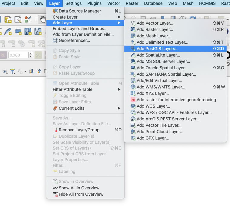
Figure 7.7: Adding a PostGIS layer in QGIS.

• In Connections add a New connection and fill in the connection details (Figure 7.8):
  • Name the connection (in this example glosis-docker).
  • Set the Host name to locaohost.
  • Add the Port details (5442)
  • Add the database name to connect to (in this example glosis). Change it to your database name if a different name has been used.
  • In Authentication move to the Basic tab and enter the default User name (glosis) and password (glosis).
  • Click on Test the connection to check if the database is accessible.
  • Click on OK.
  • Finally, in Connections, click on Connect. The system may prompt you again for the default username and password (glosis).

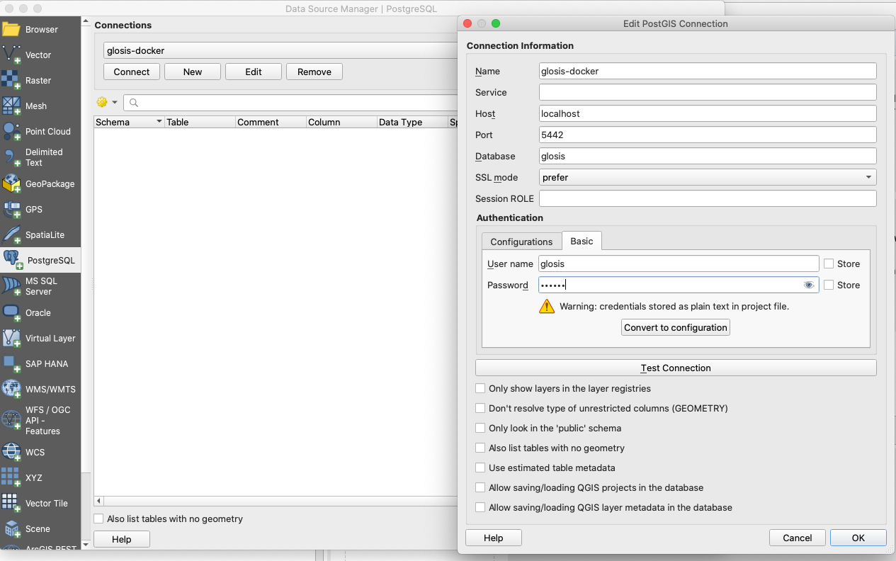
Figure 7.8: Connect to an existing database from QGIS.

Once the database has been connected, the geographic features of the database will appear under the core dropdown menu. Select plot, click on Add and the connected database will appear in your layers.

At this point, the sampling points contain only the information from the Plot Data sheet in the template. To add values for soil properties, the geographic elements of this table must be linked to the property_phys_chem table, which records such values. This can be done with an SQL query in QGIS.

• 1. Go to DB Manager in the Database main menu.
• 2. Select PostGIS in the Providers menu in the left panel and double-click on your the database connection.
• 3. Click on the SQL Window button (the second button on the top left).
• 4. Paste the following SQL query, click on the Execute button, and then click Load. Ensure that the Load as a new layer option is selected:

SELECT     
    p.name AS project_name, 
    s.site_code, 
    p2.plot_code, 
    p2.type AS plot_type, 
    p2.altitude, 
    p2.time_stamp, 
    p2.map_sheet_code, 
    p2.positional_accuracy, 
    p2."position" AS geom, 
    s2.code AS specimen_code, 
    e.type AS element_type, 
    e.upper_depth, 
    e.lower_depth, 
    o.property_phys_chem_id, 
    o.procedure_phys_chem_id, 
    r.value, 
    o.unit_of_measure_id 
FROM core.project p 
LEFT JOIN core.site_project sp ON sp.project_id = p.project_id 
LEFT JOIN core.site s ON s.site_id = sp.site_id 
LEFT JOIN core.plot p2 ON p2.site_id = s.site_id 
LEFT JOIN core.profile p3 ON p3.plot_id = p2.plot_id 
LEFT JOIN core."element" e ON e.profile_id = p3.profile_id 
LEFT JOIN core.specimen s2 ON s2.element_id = e.element_id 
LEFT JOIN core.result_phys_chem r ON r.specimen_id = s2.specimen_id 
LEFT JOIN core.observation_phys_chem o ON o.observation_phys_chem_id = r.observation_phys_chem_id  
ORDER BY p.name, s.site_code, p2.plot_code, e.upper_depth, o.property_phys_chem_id;

You will see the resulting layer with the soil attribute table (Figure 7.9) in your QGIS view. Additional attributes can be added to the table using specific SQL queries.

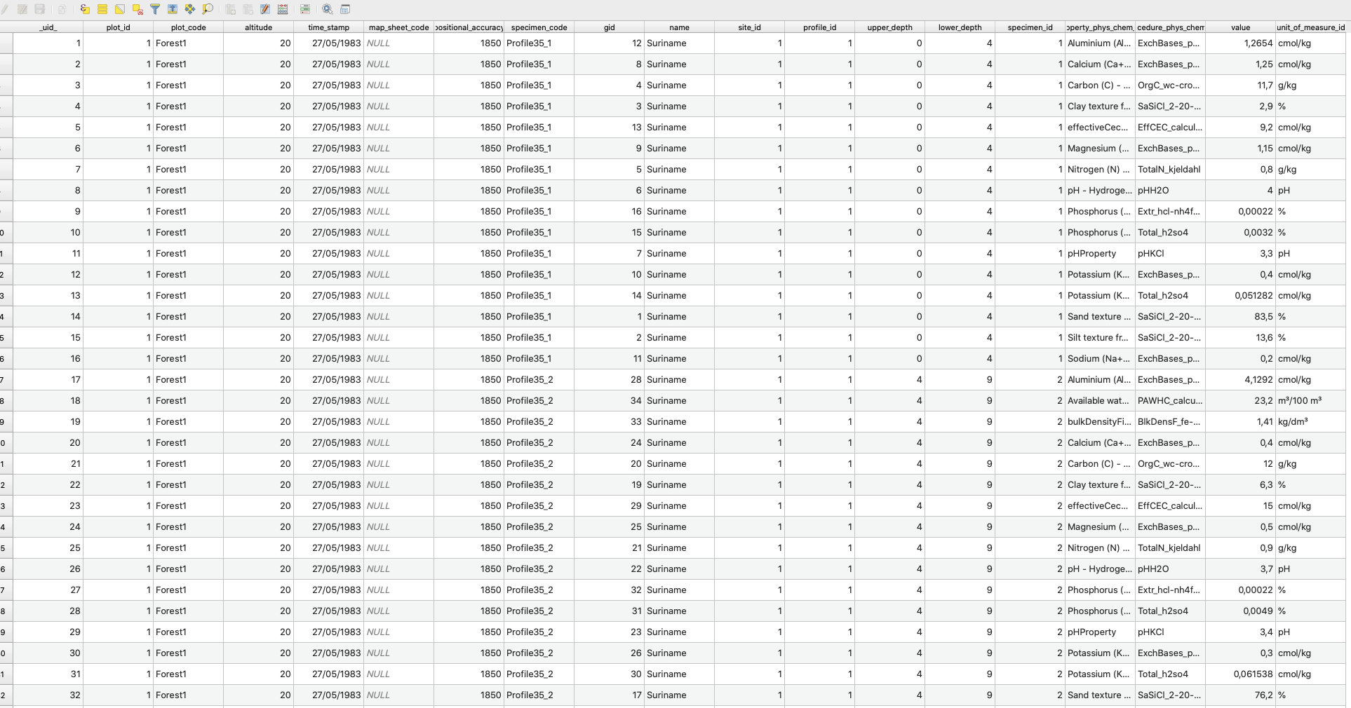
Figure 7.9: QGIS Table with soil data.